Table of contents
- Summary
- Introduction
- Context
- Partitioned loan-transfer approach
- Theory and practice of reconciliations and forecast adjustments
- Results and impacts of the treatment change
- Conclusion
- Annex 1: Partitioning step by step
- Annex 2: Impacts of forecast changes on a cohort of borrowers
- Annex 3: Alternative valuations of future repayments
1. Summary
In December 2018, we announced a decision to replace the current treatment of student loans in the public sector finance (PSF) statistics with a treatment that better reflects both the government’s and borrowers’ financial position. We will achieve this by splitting lending into two components: a genuine loan and government spending. This new approach recognises that a significant proportion of student loan debt will never be repaid by recording government expenditure related to the cancellation of student loans in the period that loans are issued rather than decades afterwards.
In the December 2018 announcement, we explained that although we had reached a decision on how best to treat student loans in principle, more work was needed to finalise detailed methodology. We also required time to construct a continuous and consistent time series from 1998, when the first income contingent loans were extended. We suggested that we would be in a position to implement the new treatment in PSF statistics in September 2019, but would aim to provide provisional estimates of the impact on headline fiscal aggregates and a methodology guide in June 2019.
We met both of these commitments, and the new treatment of student loans is now incorporated into our fiscal statistics. This article was originally published alongside the monthly Public sector finances, UK: May 2019 bulletin. It was revised and extended in January 2020 to reflect the latest developments in modelling, and address some of the frequently asked questions.
When we announced our initial decision, we estimated (based on Office for Budget Responsibility (OBR) calculations) that introducing the new treatment would increase public sector net borrowing (PSNB) by approximately £12 billion in the financial year ending (FYE) 2019. Since December 2018, we have worked with the Department for Education to develop and refine the modelling that underlies these estimates. As a result, in their March 2019 Economic and Fiscal Outlook, the OBR were able to update their estimate and report a PSNB impact of £10.5 billion in FYE 2019.
In June 2019, we provided provisional estimates of the impact on the headline fiscal aggregates of implementing the new treatment of student loans. The issuance of loans to students, together with the reduction of interest deemed to be accruing on the loan stock was provisionally estimated to increase PSNB by £10.6 billion in FYE 2019, compared with the earlier treatment of student loans.
By September 2019, we refined our early estimates. We also finished the analysis of student loan sales and set up detailed models to estimate the borrowing impact arising from the loans extended in Scotland, Wales and Northern Ireland, as well as postgraduate loans and Advanced Learner Loans. The sale in December 2018 added £1.5 billion to PSNB in FYE 2019. Combined with improved modelling, it brought the combined effect of the transition to new treatment to £12.4 billion in that year.
At the point of implementation of the new treatment of student loans in September 2019, we made one-off revisions to the PSNB and public sector net financial liabilities (PSNFL) series from FYE 1999 to FYE 2019. These revisions ensure that the historical series are shown on a basis that is consistent with the treatment change, so that the aggregates do not have step changes at the point of its implementation.
After we implemented the treatment change in September 2019, our forecasts will be updated regularly to incorporate assumption changes and to reconcile the forecast with outturn data. This methodology guide explains how the modelling is done and describes our approach to situations where:
- outturn repayment data differ from expected repayments
- economic forecasts used in estimating future repayments become outdated
- new policies are introduced that impact existing borrowers, such as a change in the repayment threshold
In all three cases, we will not go back and further revise the historical data relating to the original loan extension, but instead we will introduce the impacts at the point in time that the new information becomes available or the policy is enacted. All such updates will have an impact on loan stock values in the accounts, and so PSNFL, but only some will affect PSNB. The main principles can be summarised as follows:
- outturn repayment reconciliation will require the recording of adjustments as expenditure or revenue, which will impact PSNB
- economic forecast updates will not impact PSNB
- introduction of new policies will only impact PSNB where the loan stock value is significantly affected by the expected change in future repayments related to existing loans
This methodology guide explains the rationale for these different approaches. It also explains that in the case where the government sells tranches of student loans, it would be anticipated that the sale price would be similar to the loan stock value recorded in the PSF statistics. Where this is the case there would be no PSNB impact resulting from the sale. However, if we observe significant difference between the sale price and the loan stock value, we will record government expenditure or revenue at the time of the student loan sale. PSNB would be accordingly impacted by an amount equivalent to the difference between sale proceeds and loan stock value as estimated for PSF purposes.
Back to table of contents2. Introduction
In December 2018, we announced our decision to partition UK student loans into lending and expenditure elements. We have made this decision in consultation with the international statistical community, having carefully reviewed the treatment of student loans in economic statistics and the findings of the Treasury Select Committee and House of Lords Economic Affairs Committee (PDF, 1.61MB).
Our decision means that the treatment of student loans within public sector net borrowing and the value of the loan asset recorded on the balance sheet better reflect the government’s financial position. This is because government revenue no longer includes interest accrued that will never be paid; and government expenditure related to cancellation of student loans is accounted for in the periods that loans are issued rather than decades afterwards.
Between December 2018 and the first publication of this guide in June 2019, we modelled the main types of UK student loans on the basis of the new partitioned approach, and developed methodology for reconciling provisional and outturn data. The remainder of this article describes the partitioned approach in greater detail. We explain how partitioning works and discuss how the latest information about the economy and government policy is reflected in student loan statistics, and so the fiscal aggregates.
Some of the estimates presented in this detailed methodological guide, particularly those in Section 4 that show the expected repayments over the entire loan term, have not been updated since the original publication in June 2019. As such, they may differ slightly from those being used in fiscal statistics. We have chosen not to update the estimates with more recent forecasts for two reasons.
Firstly, this article serves as an illustrative guide to how the partitioning of student loans is done, and how it affects the fiscal aggregates. The methodological article is not meant to be a source of the latest estimates, which are available in the analytical tables published alongside the Public sector finance (PSF) bulletins.
Secondly, these estimates are periodically updated to reflect the latest information about the state of the economy (on which student loan estimates are reliant). It would be impractical to revise the guide each time these statistics get updated.
Back to table of contents3. Context
3.1. The UK student loans system
Student loans in the UK were first introduced in 1990. At first, student loans were limited in scope, only providing funds to assist students in meeting their living costs. In 1998, student-met tuition costs were introduced in UK universities, and student loans were extended in scope to include payments for tuition costs. The structure of loans was also changed at this point, with the level of repayment of the loan becoming contingent on the income of the borrower.
A number of further changes followed in the years after. The most significant of these changes, in terms of their impact on statistics, took place in 2012 when tuition fees in England rose from £3,290 to £9,000 per academic year and borrowing limits were raised accordingly. At the same time, average interest rates paid by students on the loans were increased. These changes have led to a rapid rise in the stock of student loans in recent years, and the stock currently has a nominal value1 of around £120 billion, or 6% of gross domestic product (GDP). This stock is projected, by the Office for Budget Responsibility (OBR), to rise further to nearly 20% of GDP by 2040.
A consequence of the current student loan policy is that, by design, a significant proportion of the stock of student loans will be cancelled rather than repaid. This can be for a number of reasons, but most notably because a student’s earnings may remain below the earnings threshold for the 30 years after they graduate, or may rise above it too infrequently or by too small an amount to repay both their principal and the interest on it before the loan matures.
The UK setup differs from any arrangement explicitly described in the European System of Accounts: ESA 2010 and the statistical manuals, which serve as a legal basis and international professional standards for compiling national accounts and fiscal statistics. This, and the concerns raised by the House of Commons Treasury Select Committee and House of Lords Economic Affairs Committee, led us to review how student loans should be recorded in the UK National Accounts and public sector finance statistics.
3.2. Reviews into the statistical recording of student loans
Historically, student loans were recorded as conventional loans in the UK National Accounts; the same way as any other conventional loan assets held by the UK Government and recorded at nominal value. The UK’s independent fiscal forecaster, the Office for Budget Responsibility (OBR), has argued that recording of student loans as conventional loans does not reflect the true health of the fiscal position. The National Audit Office (NAO) also investigated the sale of student loans, where it was argued, the statistical treatment did not reflect the true economic impact of the transactions. Similar concerns were raised by the House of Commons Treasury Select Committee and House of Lords Economic Affairs Committee (PDF, 1.61MB).
In response to these concerns, the Office for National Statistics (ONS) conducted a review of student loans in collaboration with Eurostat and with input from other international organisations and statistical institutes. The review focused on the compliance with the existing statistical guidance and the adequacy of the guidance in the case of income contingent loans, such as UK student loans. We identified that the treatment of student loans as conventional loans led to the following effects in the accounts:
- no recognition of expected losses at inception, and a shift of associated government expenditure decades into the future
- an overestimation of government revenue in the form of interest receivable during the life time of the loans
- an inaccurate reflection of the creditor’s (government’s) true financial position by recording a nominal value that is significantly above the true economic value of the asset
- an unrealistically favourable view of government accounts when portions of the loan book are sold, as future debt cancellation of the loans sold does not impact government expenditure
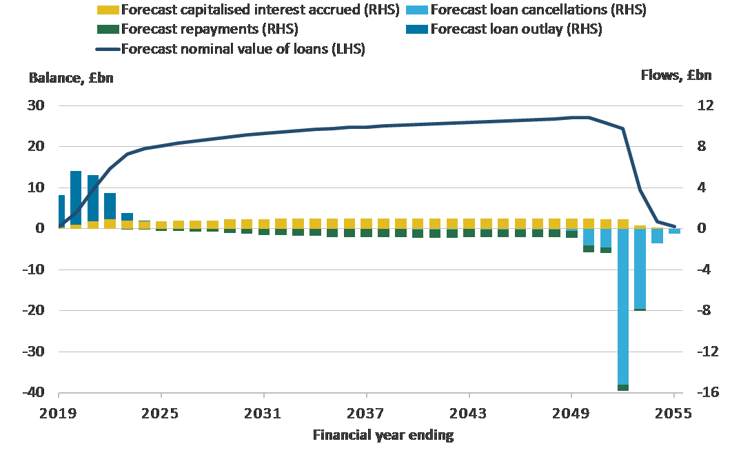
Figure 1: Under the conventional loan treatment, the loan balance is written off decades after the loans are extended
Illustrative example based on the 2018 to 2019 cohort of students, England, financial year ending 2019 to financial year ending 2056
Source: Office for National Statistics using Department for Education’s forecasts
Notes:
- By cohort we understand a group of students that receive the first part of their student loans in a given academic year.
- Flows that increase the loan balance, such as outlay and interest, are shown as positive transactions. Flows reducing the balance, such as repayments and cancellations, are shown as negative.
Download this image Figure 1: Under the conventional loan treatment, the loan balance is written off decades after the loans are extended
.png (30.5 kB) .xlsx (38.3 kB)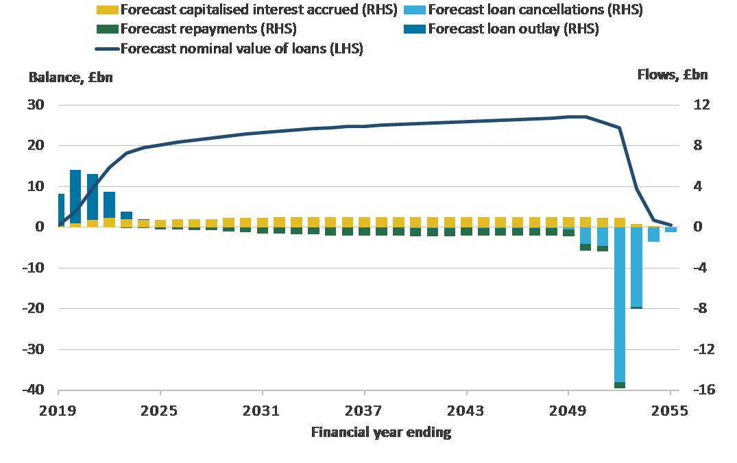
Since the European System of Accounts 2010: ESA 2010 and the associated statistical manuals are generally definitive in relation to their treatment of loans, the methodological challenges could not be addressed through a change to statistical methodology alone, without a review of the economic substance of the UK student loans and similar income contingent instruments. We noted that the UK student loans, although loans in a legal sense, did not fully meet the criteria of a loan as defined in ESA 2010. Therefore, the ONS and Eurostat engaged with other international statistical organisations and national statistical institutes on the most appropriate alternative recording.
3.3. ONS review outcome and Eurostat’s bilateral advice
Following the engagement with the international statistical community, the Office for National Statistics (ONS) and Eurostat reflected on the contributions received and concluded that the best way to record UK student loans in the national accounts is to treat part as loans, since some portion will be repaid, and part as capital transfers, since some will not. This partitioned loan-transfer approach is considered best to reflect the economic substance of income contingent loans, including the UK student loans, from the perspectives of both the government and students.
The partitioned loan-transfer approach takes the concept introduced in paragraph 20.121 of the European System of Accounts 2010: ESA 2010 and applies it to a loan book, as distinct from an individual loan:
“Loans (F.4) include, in addition to loans to other government units, lending to foreign governments, public corporations, and students. Loan cancellations are also reflected here with a counterpart entry under capital transfer expenditure. Loans granted by government not likely to be repaid are recorded in the ESA as capital transfers, and are not reported here.”
The basic idea is that a portion of the student loan outlay is considered to be a capital transfer to the borrower (this can be thought of as the government cancelling this portion of the loan at inception), with the remaining portion treated as a genuine loan asset or liability. Adopting the partitioned loan-transfer approach addresses most of the issues with the current treatment. In support of the approach, Eurostat issued an official letter recognising the need to treat the extension of loans unlikely to be repaid as government expenditure at inception.
While the overall treatment of UK student loans was announced in December 2018, questions of methodological nature remained, such as:
how to estimate what proportion of the outlay should be recorded as government expenditure
how to reconcile initial estimates with outturn statistics
what to record if these estimates change because of policy decisions or macroeconomic conditions
The remainder of this article describes the partitioned approach in greater detail. We explain how partitioning works and discuss how the latest information about the economy and government policy will be reflected in student loan statistics and so the fiscal aggregates.
Notes for: Context
- Nominal value is defined as the principal extended plus interest accrued, less repayments and debt cancellations.
4. Partitioned loan-transfer approach
4.1. Overview of the approach
Under the partitioned loan-transfer approach, the extension of loans to students is seen as a combination of lending and transferring funds. Conceptually, the transfer is seen as forgiveness of loans that are unlikely to be repaid at inception. In simple terms, lending should capture student loans that are expected to be repaid; while the transfer should capture those that are not. Those student loans that are expected to be repaid would give rise to accrued interest, just as any conventional loans. In contrast, student loans recorded as a transfer at inception are not financial assets for the creditor and cannot be directly associated with any interest or repayments. These basic facts can be summarised as follows:
outlay must be partitioned into the lending and transfer elements
interest must accrue only on the proportion of outlay recorded as lending
repayments must go towards student loans recorded as lending
the model must avoid the inherent need to cancel or write off loans at maturity
The application of the three principles immediately raises a question of how to approach loans that are only expected to be repaid partially. By way of example, one could imagine a situation whereby a borrower has repaid the capitalised interest but not the principal, which is cancelled at the end of the loan term. The issue for national accountants is that if the original loan is recorded as a transfer, no interest should be accruing, and no repayments should be made because of the unrequited nature of the transfer at inception. If, on the other hand, the transaction is recorded as a standard loan, the cancellation of the principal is shifted decades into the future.
This leads to the conclusion that the partitioning should be based not on the number of individual loans and the binary outcome of them being repaid at maturity or not, but on the value of the total outlay and the associated capitalised interest that are expected to be repaid. Put differently, an individual student loan can be partitioned between the lending and transfer elements if it is not expected to be repaid in full. The part of the student loan reported as a standard loan must be expected to be fully repaid at maturity, to avoid the need to cancel the outstanding balance decades from inception. In practice, of course, while partitioning at an individual level may be estimated to create aggregate statistics, economic analysis is more appropriate at or above the cohort level, similarly to the cases of insurance and standardised guarantees.
Under the partitioned loan-transfer approach, only the loan component should accrue interest and so the reported interest on the total loan book needs to be adjusted in accordance with the calculated transfer component; in what follows we call this adjusted interest the “modified interest”. The loan component of the outlay and the cumulative modified interest minus repayments, comprises the modified loan balance.
UK student loans are extended in separate instalments at the start of academic terms. Most undergraduate students in a given cohort study for three academic years; some enrol on longer study programmes or defer their studies, meaning that for each student, or cohort, the outlay has to be partitioned over several years and many terms1.
A further complication is that both the interest rate applied to the balance and the repayment amounts in each time period are contingent on the borrower’s income. Both of these variables therefore need to be forecast using economic models. The forecast approach is conceptually consistent with estimation of the value of insurance, standardised guarantees and pensions, which all serve as useful examples of broadly similar methods of deriving present values in statistics.
4.2. Inputs into national accounts model: student loan forecasts
The need to produce accurate student loan forecasts is not new, nor is it unique to national accounts. The financing of the higher education system is reliant on that information, which informs the budgetary process and the amount of funds made available to the Department for Education (DfE, which took over responsibility for higher and further education from the dissolved Department for Business, Innovation and Skills in 2016) and the devolved administrations in Scotland, Wales and Northern Ireland. These administrative purposes require forecasts of future repayments and interest, which are important inputs to the partitioned loan-transfer model.
The present generation of forecasting models, which could be used as a basis for producing statistical estimates, dates back to a period between 2013 and 2014 when the National Audit Office (NAO) (PDF, 396.2KB), Public Accounts Committee (PAC) (PDF, 1,009KB) and the Business, Innovation and Skills Committee (BISCOM) (PDF, 1.92MB) separately considered the student loan repayment system and made significant recommendations. Improved forecasting methods were put in place in response to these recommendations.
The responsibility for running the models now rests with DfE, and the published outputs are designated official statistics and produced in accordance with the Code of Practice for Statistics. The inputs come mostly from the Office for National Statistics (ONS) data and the independent Office for Budget Responsibility (OBR) projections on macroeconomic determinants, as well as historical data on student loan performance provided by the Student Loans Company. The devolved administrations produce their own forecasts.
Presently, four separate economic models are used to produce the forecast, namely the student loan outlay model, the student loan repayment model, the student numbers model and the Advanced Learner Loans model. The modelling is done for a sample of individual borrowers, which form the whole student loan borrower population and could also be grouped into cohorts. While economic analysis may be far more meaningful at aggregated, cohort or population levels, individual-level modelling has a number of properties that are useful for loan-transfer partitioning in the national accounts. Most importantly, it allows us to model interest rates associated with the individual borrowers, which vary with individuals’ earnings in the case of some loan plans.
The outputs from these models are used for both statistical and administrative purposes. The forecasts feed into the production of DfE’s financial statements, audited by the NAO. In a similar way to the fiscal statistics, the financial statements compiled in accordance with the public accounting standards attempt to estimate the cost of future loan cancellations. This measure, known as the Resource Accounting and Budgeting (RAB) cost, is used to inform the amount of funds made available to DfE.
The RAB cost in DfE’s financial statements differs from the capital transfer at inception of loans recorded in the national accounts. Both the RAB cost and the ONS partitioning capital transfer estimate the portion of loan outlay provided over the financial year, which is not expected to be repaid. They differ in the way they discount future repayments in order to estimate the current value of future forecast repayments.
The RAB cost values future repayments by taking into account the effect of inflation and the estimated cost of government borrowing over time, whereas under the ONS partitioned loan-transfer model, future repayments are valued by taking into account the interest rates charged on student loans. Therefore, where a borrower’s interest rate is higher than the combined impact of inflation and government borrowing, the repayments are discounted by a higher value under the partitioned loan-transfer model so the partitioning capital transfer will be higher than the RAB cost.
In Table 6 of Annex 3, we provide a descriptive overview of the main differences between the statistical value of future repayments, calculated under the ONS partitioned loan-transfer methodology, and the accounting value of future repayments, calculated through DfE’s RAB cost.
Having employed economic models to create repayment and interest rates projections, we can build on the principles laid out in Section 4.1 and use algebra to derive the national accounts outputs: expected loan balance throughout the entire period to maturity, and, in the next step, partitioning at inception. The next section provides a general overview of the model, with a detailed description of the calculations located in Annex 1.
4.3. Results in a closed group: stylised example
The best way to illustrate how the model works is to apply it to one cohort of students. Being a closed group, a cohort has a set outlay period and loan term end, allowing us to visualise the trajectories of all relevant variables between loan extension to maturity. Of course, one cohort would not convey the sense of scale of the loan book and for that reason, Section 6 presents the population level estimates.
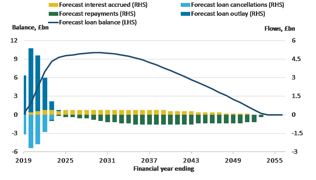
Applying the principles described in the previous subsections to borrowers in the 2018 to 2019 cohort yields a very different picture to that presented in Figure 1. The Office for National Statistics (ONS), using early estimates from the Department for Education (DfE), forecasts that £16 billion of loans will be extended to this cohort. Under the partitioned loan-transfer approach, the outlay (£16 billion) is partitioned between lending in national accounts terms (£8 billion) and transfers (£8 billion).
Modified interest (£10 billion) only accrues on the former component; therefore, it is lower than the amount recognised in the national accounts under the conventional loan treatment (£31 billion). The ratio of modified interest to conventional interest (approximately 1:3) is considerably lower than the ratio of modified lending to full outlay (approximately 1:2). This is because of the compounded interest, which quickly increases the nominal balance when the loans are not being repaid.
In the overview of the partitioned loan-transfer approach we stated that there should be no inherent need to write-off outstanding balance at maturity. In other words, student loans have to be partitioned in such a way that the lending component with the associated modified interest is fully repaid. With none of the projected repayments (£18 billion) going towards the transferred amounts, the following identities hold over the lifetime of the loans:
(1)
(2)
(3)
The partitioned model can be contrasted with the conventional loan treatment. For the same cohort, DfE estimates that the £16 billion of loans extended to students will give rise to £30 billion of (non-modified, nominal) interest. Of the total cumulative liability of £46 billion, £18 billion are expected to be repaid and £28 billion would be written off at the end of loan term, over 30 years after the loan extension (see Figure 1).
Figure 2: Under the partitioned loan-transfer approach, a portion of the loan outlay is written off when the loans are extended
Illustrative example based on the 2018 to 2019 cohort of students, England, financial year ending 2019 to financial year ending 2056
Source: Office for National Statistics using Department for Education’s forecasts
Notes:
- By cohort we understand a group of students that receive the first part of their student loans in a given academic year.
Download this image Figure 2: Under the partitioned loan-transfer approach, a portion of the loan outlay is written off when the loans are extended
.png (33.6 kB) .xlsx (38.6 kB)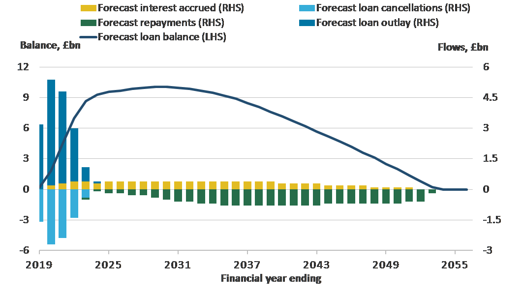
Notes for: Partitioned loan-transfer approach
- The students become liable for the amounts extended at the term start. We therefore consider outlay a good proxy for recording lending on an accrual basis.
5. Theory and practice of reconciliations and forecast adjustments
5.1. Rationale for making statistical adjustments
The model projects repayments and interest accruals over several decades into the future. With such a lengthy forecast horizon, the estimates are sensitive to changes in assumptions. It can be expected that, because of changes in the macroeconomic conditions or government policy, there will inevitably be discrepancies between the forecasts and the outturn. Even before the actual data can be collected, the expectations themselves will have most likely moved on.
The revised expectations may no longer support the modelled loan stock and interest accruals trajectories (themselves a function of the loan stock and earnings). That is, less money could be expected in repayments, meaning the loan stock – if not adjusted – will not be fully repaid at maturity and more interest will accrue than can be repaid.
Figure 3 demonstrates a scenario using the cohort of students starting in 2018, a scenario where repayment expectations worsen in the financial year ending (FYE) 2026.
Figure 3: Under the partitioned loan-transfer approach, when repayment expectations worsen, the loan balance will not fall to zero if it is not updated
Illustrative example based on the 2018 to 2019 cohort of students, England, financial year ending 2019 to financial year ending 2056

Source: Office for National Statistics using Department for Education’s forecasts
Notes:
- By cohort we understand a group of students that receive the first part of their student loans in a given academic year.
Download this image Figure 3: Under the partitioned loan-transfer approach, when repayment expectations worsen, the loan balance will not fall to zero if it is not updated
.png (46.2 kB) .xlsx (39.1 kB)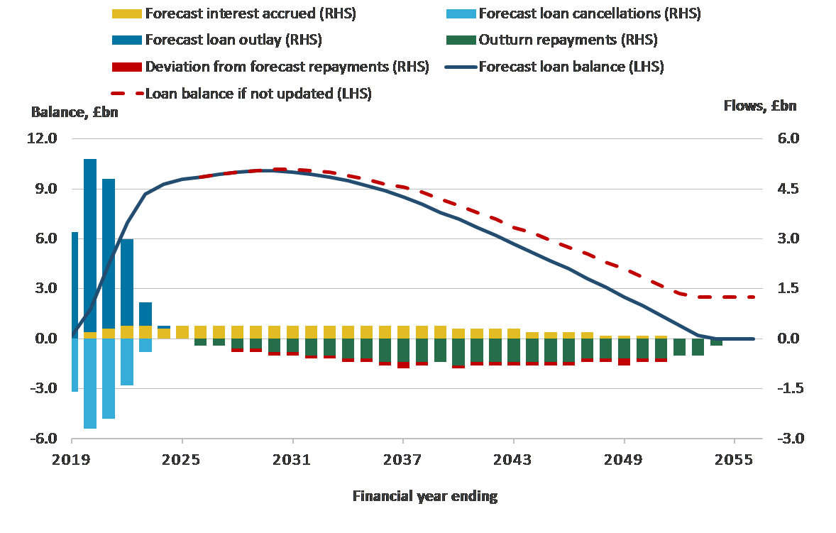
Similarly, should earnings growth accelerate, more borrowers would be able to repay and reduce the unadjusted stock to zero before they stop making actual repayments to the Student Loans Company. Avoiding these effects requires statistical adjustments to be recorded whenever expectations change. In practice, changes to expectations would have to be applied to the entire population of borrowers, including those for whom partitioning had been done in the previous time periods. As a parallel, actuarial estimates of defined benefit pension entitlements are also adjusted in the national accounts each time the new valuation (based on updated assumptions) becomes available.
5.2. Distinction between forecast and outturn reconciliation
Having briefly illustrated the need to record some sort of adjustments, it is useful to distinguish events that should lead to complete revaluation of the loan stock and those whose effect should be limited to the time period in which the discrepancy is observed.
Let us consider two contrasting scenarios. There is normally a time lag before a shock in the financial markets is transmitted to the labour market. When an economic downturn starts, there may be no significant discrepancy between the forecast and outturn in the first year. This does not mean that there are no adjustments to record: the borrowers are now expected to repay less in subsequent years.
The economic value of the loan book, being a forward-looking measure, is certain to shrink as the new, worse expectations of future earnings growth are formed. With less expected to be repaid, the original loan stock trajectory can no longer be supported, and a statistical adjustment needs to be applied to reduce the value of the stock, as shown in Figure 4. Later in this article, we refer to this type of adjustment as forecast reconciliation.
Figure 4: Under the partitioned loan-transfer approach, the loan balance is adjusted downwards when repayment expectations worsen, so that it falls to zero by the end of the loan term
Illustrative example based on the 2018 to 2019 cohort of students, England, financial year ending 2019 to financial year ending 2056

Source: Office for National Statistics using Department for Education’s forecasts
Notes:
- By cohort we understand a group of students that receive the first part of their student loans in a given academic year.
Download this image Figure 4: Under the partitioned loan-transfer approach, the loan balance is adjusted downwards when repayment expectations worsen, so that it falls to zero by the end of the loan term
.png (47.9 kB) .xlsx (38.0 kB)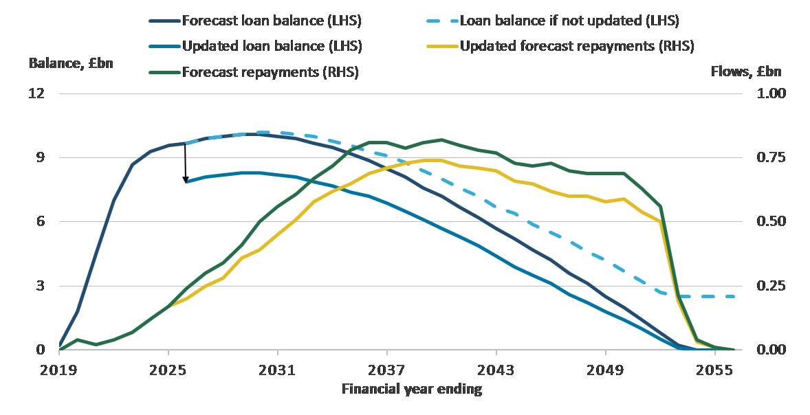
A very different example would be where no fundamentals change but a discrepancy is observed between expected and actual repayments. Indeed, the nature of economic models is such that there will always be some error between the expected and actual outcomes.
Figure 5 demonstrates a scenario where outturn repayments differ from forecasts from FYE 2026 onwards. Yet the mere existence of an error term in the present (unless indicative of a persistent bias) conveys no information about the trajectory of the relevant variables in the future. The statistical adjustments required in this case would therefore be much smaller, reconciling the observed repayments with those expected but not seeking to change the residual value of the loan book. This type of adjustment is called outturn reconciliation hereafter.
Figure 5: Under the partitioned loan-transfer approach, outturn repayments may differ from forecast repayments without creating the need to adjust the loan balance
Illustrative example based on the 2018 to 2019 cohort of students, England, financial year ending 2019 to financial year ending 2056

Source: Office for National Statistics using Department for Education’s forecasts
Notes:
- By cohort we understand a group of students that receive the first part of their student loans in a given academic year.
Download this image Figure 5: Under the partitioned loan-transfer approach, outturn repayments may differ from forecast repayments without creating the need to adjust the loan balance
.png (33.7 kB) .xlsx (36.5 kB)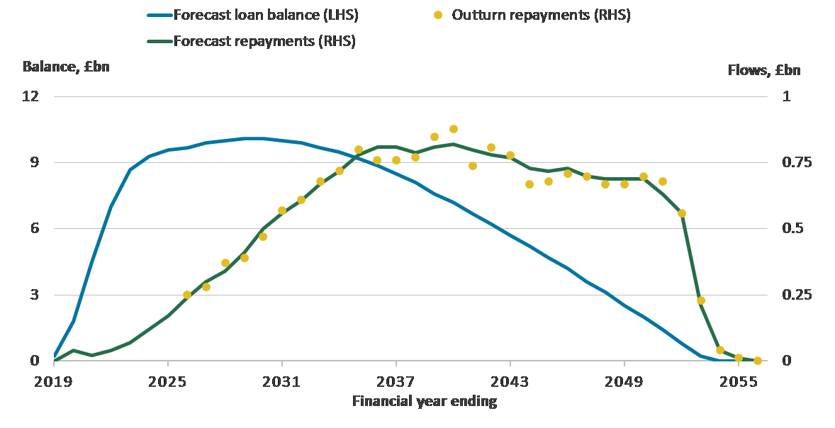
Having illustrated the pure adjustment mechanisms, it is useful to consider a mixed scenario where over time, the outturn data suggest a persistent bias in the repayment forecast. The response will be a combination of the reconciliation approaches discussed earlier.
Firstly, the assumptions (and potentially the model specifications) have to be revisited to produce a new forecast, and so a new stock value, which should correct the systematic element of the errors. Secondly, any remaining discrepancies will be reconciled in the same way as outturn reconciliation, through recording revenue or expenditure at the time when they are observed. The following sections add more technical details to the explanation of this process.
Figure 6: High-level adjustment process in cases where estimates have been biased
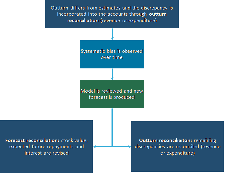
Source: Office for National Statistics
Download this image Figure 6: High-level adjustment process in cases where estimates have been biased
.png (19.5 kB)
5.3. Outturn reconciliation
It is important to remember that it is the validity of the long-term repayment forecast that matters for the loan stock value (itself a discounted value of expected future repayments), and consequently for accrual of modified interest. Therefore, the forecast should ensure that in the long term, the sum of the modelled future repayments should be approximately equal to the sum of outturn repayments. The stock value will then hold even if in a given period, the repayments are not exactly as predicted. In other words, in the short term, the outturn repayments can be higher or lower than expected.
While we do not necessarily need to revalue the loan stock, unforeseen discrepancies in repayments must nonetheless be accounted for. Assuming no new lending takes place, the difference in the loan balances between the present and the past periods must be explained by expected repayments, which decrease the outstanding balance, and modified interest, which increase the outstanding balance.
If cash repaid by the borrowers is consistent with movements in the estimated stock value and modified interest accrued over the time period, no further adjustments are needed. Otherwise, a further debt cancellation or revenue equal to the discrepancy between actual repayments on one side, and the reduction in the modified loan stock less interest payable on the other side, has to be recorded as a capital transfer in accordance with Eurostat’s advice.
Recording the unforeseen element of repayments as a capital transfer (either receivable or payable) ensures that over the entire loan term, public sector net borrowing (PSNB) calculated an accrual basis reflects the true cost to the government of providing the loans.
Table 1 uses the example of the same notional cohort as shown in Figure 5 and demonstrates a simplified accounting treatment of that cohort in the FYE 2040, assuming the outturn data for that year have become available.
Table 1: Outturn reconciliation under the partitioned loan-transfer approach, illustrative sequence of accounts based on the 2018 to 2019 cohort of students
| England, £ million | |||||
|---|---|---|---|---|---|
| Government sector balance sheet on 1 April 2039 | |||||
| Assets | Liabilities | ||||
| Government’s cash balance | AF.2 | X | |||
| Government’s modified loan stock | AF.4 | 7650 | |||
| Net worth | BF.90 | X+7650 | |||
| Non-financial transactions | |||||
| Uses | Resources | ||||
| Interest accruing on loan stock | D.4 | 355 | |||
| Unforeseen debt cancellation | D.9 | 50 | |||
| Net borrowing | B.9g | 355 | |||
| Financial transactions | |||||
| Δ(Assets) | Δ(Liabilities) | ||||
| Repayments by borrowers | F.2 | 764 | |||
| Reduction in loan stock value | F.4 | -459 | |||
| Net borrowing | B.9f | 305 | |||
| Other economic flows | |||||
| Revaluation | - | ||||
| Government sector balance sheet on 31 March 2040 | |||||
| Assets | Liabilities | ||||
| Cash balance | AF.2 | (X+764) | |||
| Loan balance | AF.4 | 7191 | |||
| Net worth | BF.90 | (X+764)+7191 | |||
| Source: Office for National Statistics using Department for Education’s forecasts | |||||
| Notes: | |||||
| 1. By cohort we understand a group of students that receive the first part of their student loans in a given academic year. | |||||
Download this table Table 1: Outturn reconciliation under the partitioned loan-transfer approach, illustrative sequence of accounts based on the 2018 to 2019 cohort of students
.xls (63.5 kB)We discussed that over time, it may become evident that a systematic bias exists. The fundamental solution would be to reassess the validity of the forecast (including inputs into the model) to eliminate the apparent bias and produce a revised forecast.
However, the new forecast will apply from the period when it is produced, leaving a back series of historical estimates that may be suffering from bias. Although one could want the updated stock value to apply from an earlier period, it may not be feasible to identify when exactly the bias first arose and produce forecasts from that point; nor may it be desirable, for both conceptual and practical reasons, to use the information revealed in the present to value financial instruments in the past1. Therefore, prior to the moment when the new forecast is produced, the outturn reconciliation method will apply and the stock value will not be adjusted. It will ensure that the cumulative PSNB impact will be correctly recorded, albeit the historical stock values, and so government and household sectors’ net worth could remain under- or over-estimated.
5.4. Forecast reconciliation
General principle
Fundamentally, forecast reconciliation differs from outturn reconciliation in that a new set of expectations must underpin the value of the loan stock. That new value, together with the associated interest payable by the students, must be incorporated into fiscal statistics to avoid a situation where either repayments continue to flow in after the original (unrevised) loan stock has been deemed repaid, or the unrevised stock is never fully repaid if less cash ultimately comes in (Figures 3 and 4).
Algebraically, the statistical adjustment needed to reconcile the accounts with the balance sheet is simply the difference between the loan stock under the old expectations, and the loan stock under the new expectations. From then on, the interest accrued on the balance will also change, to be consistent with both the balance itself and with potential revisions to inflation and earnings expectations, to which the interest rate is linked.
Estimating the value of the statistical adjustment is easier than determining how it should be recorded in fiscal statistics. New information about the historical repayments or evolving expectations of the future economic conditions may require updating the forecast, and with it, loan stock valuation. Changes to terms and conditions of the existing loans will also instigate a need to compile a new forecast. It is important to make a distinction along two dimensions:
between new information about the economy and deliberate acts of government intervention
within the category of government interventions, between those that significantly change the loan stock value through expectations of future repayments and those that affect the stock value predominantly through a change in the discounting factor
Statistical recording of revised economic expectations
The former criterion is relatively straightforward. Paragraph 6.14 of the European System of Accounts: ESA 2010, among examples of “other changes in volume not elsewhere classified concerning financial assets and liabilities” lists “changes of life insurance, annuity entitlements and pension entitlements due to changes in demographic assumptions”. Effectively, this applies to all those financial instruments in the system of national accounts (other than income contingent loans not envisaged by ESA 2010) where economic modelling is applied in establishing the value of the financial instrument.
This is expanded on in Chapters 6 and 17 of ESA 2010, where a distinction is made between demographic and economic assumptions:
“The liabilities to policy holders and beneficiaries change as a result of transactions, other volume changes and revaluations. Revaluations are due to changes of key model assumptions in the actuarial calculations. Those assumptions are the discount rate, the wage rate and the inflation rate.” (Chapter 6, paragraph 6.61)
“Revaluations are due to changes of key model assumptions in the actuarial calculations. These assumptions are the discount rate, the wage rate and the inflation rate. Experience effects are not included here unless it is not possible to identify them separately. Other changes in actuarial estimates are more likely to be recorded as other changes in volume of assets. The effects of price changes due to the investment of the entitlements are recorded as revaluations appearing in the revaluation account.
“When the demographic assumptions used in the actuarial calculations are changed, they are recorded as other changes in the volume of assets.” (Chapter 17, paragraphs 17.159 to 17.160)
In accordance with this guidance, we will record changes in economic assumptions either as revaluation, or as other changes in volume, depending on their exact nature.
Statistical recording of policy interventions
Having briefly made the case for treating new information as a non-transactional change in balances, it is useful to turn to policy interventions.
First, the treatment must depend on whether the policy change affects the existing loans, or only applies to loans that will be expended in the future. In the latter case, no statistical adjustments need to be recorded in the present. When the loans under the new policy are ultimately extended to future cohorts of students, the values of modified lending and transfers recorded in the corresponding time period will be estimated on the basis of the new terms.
On the other hand, policies that affect existing borrowers must be reflected in the existing loan stock. Similar to the case of economic assumption changes, the value of the adjustment must equate to the difference between the pre- and post-intervention loan balance (net of the impact of any new lending, interest and repayments). But unlike the earlier case, such a change will not always be recorded as revaluation. As a general guiding principle, paragraph 1.66 of the ESA 2010 defines transaction as follows:
“A transaction is an economic flow that is an interaction between institutional units by mutual agreement or an action within an institutional unit that it is useful to treat as a transaction, because the unit is operating in two different capacities.”
Negotiated changes to terms and conditions of existing financial instruments are generally recorded as transactions. In most cases, the negotiation would take place between creditor and debtor, however, as paragraph 17.154 of ESA 2010 clarifies in relation to government pension liabilities, “if changes (…) are agreed by the parliamentary authorities, this is recorded as if it were negotiated.” This clarification is consistent with the general principle that most lawful actions of the government are recorded as transactions even if there is no direct and explicit agreement with the counterparty. The most trivial example of why that is the case is the government’s ability to impose taxes and create the associated tax liability, which is deemed to be done by mutual agreement with the taxpayers:
“The definition of a transaction implies that an interaction between institutional units be by mutual agreement. When a transaction is undertaken by mutual agreement, the prior knowledge and consent of the institutional units is implied. The payments of taxes, fines and penalties are by mutual agreement, in that the payer is a citizen subject to the law of the land. However, uncompensated seizure of assets is not regarded as a transaction, even when imposed by law.” (Paragraph 1.79, ESA 2010)
Eurostat’s advice letter adds further detail to this idea by arguing that policy interventions need to be recorded as transactions affecting net borrowing of the government sector if they are significant and have an impact on the amounts the government can expect to receive in repayments. The reference to “significant” changes serves two purposes.
Firstly, the national accounts estimates are generally produced on an accrued-to-date basis and should not aim to predict future changes to terms and conditions when such changes are not an outcome of existing policies. Some of these changes could be rather routine, albeit not automatic. In these situations, it can often be problematic to decide what constitutes a new, or substantially amended government policy, and what is merely a continuation of the existing policies. For instance, the government might choose to increase the repayment threshold in line with inflation every year, in a similar way as it does for Income Tax allowance. While such a change could be widely anticipated, it is not explicitly stated in the terms and conditions of all student loans.
A change like an inflation indexation of the repayment threshold will generally have a small impact on the loan balance (a stock measure) but could have significant implications for public sector net borrowing (PSNB, a flow measure) if it was recorded as a capital transfer, because of the sheer size of the loan book. There are other parameters of income contingent loans that might potentially be amended on a fairly regular basis, and it would impair the interpretation of the statistical aggregates if all of them were to be transmitted into PSNB or the household sector’s savings ratio.
There is another consideration too. Under the partitioned approach, the loan stock is valued by discounting expected future repayments, where the discounting factor is based on the interest rates faced by the borrowers. This means that if the government were to reduce interest rates on existing loans, it could achieve an increase in loan value and a reduction in estimated debt cancellation at inception without changing the undiscounted value of repayments for borrowers who do not repay in full. The increase in lending is a logical consequence of the loan affordability concept built into the partitioned loan-transfer approach, which, in turn, follows the ESA 2010 definition of a loan: for a transaction to be considered lending, the borrower must be able to repay the full amount borrowed, with interest, by the end of the loan term. As with mortgages, the lower the interest, the more can be borrowed.
For those borrowers who will not repay the full amount, this effect reprofiles government expenditure by reducing debt cancellation at inception and subsequently reducing government revenue from interest. As such, it may not change the cumulative impact on net borrowing over the entire loan term but has pronounced short-term effects. If the government were to reduce interest rates associated with existing loan stock, and if a capital transfer were to be recorded, it would have to be treated as government revenue at the point of the policy enactment, even though in the longer-term revenue from repayments would decrease.
To make sure that these properties of the partitioned approach do not adversely affect the interpretation of the fiscal aggregates, the treatment of the policy interventions should depend on the nature of those interventions. For example:
policy changes only affecting future borrowers will not require statistical adjustments in the present, and future partitioning associated with those loans will be done on the basis of new terms and conditions
amendments to terms and conditions of existing loans that do not significantly alter the loan stock value by changing amounts the government is expected to receive, will be recorded as other economic flows and will not affect PSNB
interventions significantly altering loan stock value through changing expectations of future repayments (associated with existing loans) will give rise to capital transfers and will affect PSNB
These principles will also apply to packages of changes, which may combine elements that alter expectations of future repayments as well as changes to the interest rate, which may predominantly affect the value of the loan through discounting. It would be impractical to attempt to separate the various elements of the change package.
Indeed, even if such a separation were done, the order in which the individual elements of the package are modelled may affect the relative size of the effects. For these reasons, if a change package significantly alters the amounts of expected future repayments associated with existing loans, we will record the cumulative effects of the entire package as a capital transfer that will be affecting PSNB.
Table 2 shows the accounting treatment of both the routine economic assumptions updates, and policy interventions.
Table 2: Forecast reconciliation under the partitioned loan-transfer approach, illustrative sequence of accounts based on the 2018 to 2019 cohort of students
| England, £ million | |||||
|---|---|---|---|---|---|
| Government sector balance sheet on 1 April 2020 | |||||
| Assets | Liabilities | ||||
| Government’s cash balance | AF.2 | Y | |||
| Government’s modified loan stock | AF.4 | 8265 | |||
| Net worth | BF.90 | Y+8265 | |||
| Non-financial transactions | |||||
| Uses | Resources | ||||
| Interest accruing on loan stock | D.4 | 470 | |||
| Cancellation of new loans extended | D.9 | 711 | |||
| Major terms and conditions change | D.9 | 575 | |||
| Net borrowing | B.9g | -816 | |||
| Financial transactions | |||||
| Δ(Assets) | Δ(Liabilities) | ||||
| Outlay less repayments by borrowers | F.2 | -1323 | |||
| Transactional change in loan stock | F.4 | 507 | |||
| Net borrowing | B.9f | -816 | |||
| Other economic flows | |||||
| Demographic assumption change | K.5 (AF.4) | -104 | |||
| Economic assumptions change | K.7 (AF.4) | -190 | |||
| Government sector balance sheet on 31 March 2021 | |||||
| Assets | Liabilities | ||||
| Government’s cash balance | AF.2 | (Y-1323) | |||
| Government’s modified loan stock | AF.4 | 8478 | |||
| Net worth | BF.90 | (Y-1323)+8478 | |||
| Source: Office for National Statistics using Department for Education’s forecasts | |||||
| Notes: | |||||
| 1. By cohort we understand a group of students that receive the first part of their student loans in a given academic year. | |||||
| 2. The household sector sequence of accounts is symmetrical and is not shown here for brevity. | |||||
Download this table Table 2: Forecast reconciliation under the partitioned loan-transfer approach, illustrative sequence of accounts based on the 2018 to 2019 cohort of students
.xls (64.5 kB)5.5. Sales of student loans
The final reconciliation mechanism we need to consider is that associated with a student loan sale. In 2017, the government completed the first sale of parts of the income contingent student loan portfolio. A further sale has taken place since, and more could be conducted in the future. The sales transfer the right to benefit from future repayments to private investors, in exchange for an agreed amount of cash at the point of sale.
The present value of loans is subject to uncertainty. The level of repayments over the loan term is contingent on borrowers’ future income; additionally, the value to the government or investors of holding student loans as an asset may differ from the statistical estimate of their value. For these reasons, it can be expected that the sale proceeds may differ from the estimated value of the loans; these numbers differ inherently in what they represent.
The proceeds achieved in a sale are received from investors. The value that investors place on the sale is informed by their view of the present value of the future cashflows expected to be repaid from the sold loans, taking into account their cost of capital, and the perceived risk of those future cash flows (the government’s value for money assessment considers similar factors when judging if there is more value to the government in selling or retaining loans). In contrast, as set out earlier, the national accounts value is an estimate of the statistical value of future repayments based on the loan balance, principle, and interest expected to be fully repaid before the loans are written off.
The proceeds can either be lower, reflecting uncertainty associated with future revenues, or higher, for example, if investors expect future repayments to exceed the amounts estimated by the Department for Education (DfE), and subsequently used to value loan stock in the UK National Accounts. Given these differences, the reconciliation between the sale proceeds and the statistical value of future repayments is designed to recognise the impact of the sale in the national accounts. It is not designed to assess the value for money of any given loan sale; the government separately considers the value for money of each sale using various measures. Further details can be found in the reports submitted to parliament following the sale in 2017 (PDF, 776.8KB) and in 2018.
In Table 6 of Annex 3, we provide a descriptive overview of the main differences between the ONS partitioned loan-transfer methodology, used to calculate the statistical value of future repayments and the methodology used for the government’s value for money assessment of loan sales.
Where no significant difference exists between the sale price and the loan stock value, as estimated for national accounts purposes, likely reflecting the risk premium, then the sale will be recorded as a financial transaction with no impact on public sector net borrowing (PSNB). This is in accordance with the European System of Accounts 2010: ESA 2010 guidance:
“When an existing loan is sold to another institutional unit, the write-down of the loan, which is the difference between the redemption price and the transaction price, is recorded under the revaluation account of the seller and the purchaser at the time of transaction.” (Paragraph 6.58)
While a sale may achieve the policy objectives set by the government, it could nonetheless represent a loss or a gain of future revenue that has not been accounted for by partitioning at inception, as estimated using the national accounts discount rate, which often differs from a market discount rate. We will therefore analyse each sale and where we judge that the price is significantly different from the value recorded in the national accounts balance sheet, we will, in accordance with the advice provided by Eurostat (PDF, 91.25KB), record a capital transfer. The transfer will affect PSNB by imputing expenditure equal to the difference in value between the realised sale proceeds and our estimate of the corresponding loan asset’s value, ensuring that the expenditure associated with extending the loan is fully captured in government accounts.
Notes for: Theory and practice of reconciliations and forecast adjustments
- Let us consider an example of share valuation. The share price will generally go up or down when information about the company’s performance is disclosed. That moment is generally later than the periods when profits or losses have been built up.
6. Results and impacts of the treatment change
6.1. Quality of the data included in this section
While student loans extended after 1998 have a set of common features, they vary in specific terms and conditions; the variation exists between cohorts within broad types such as Plan 1, and indeed between loans extended to students domiciled in England, Scotland, Wales and Northern Ireland.
Owing to the complexities of estimating how much of the loan outlay, interest and repayments are associated with each of the different types of student loans in the UK, the estimates and their impacts on the fiscal aggregates that are presented in this section are provisional. The aggregate figures in this article were improved upon when we implemented the new treatment of student loans in the public sector finance (PSF) statistics in September 2019.
The independent Office for Budget Responsibility (OBR), in its Working paper on student loans and fiscal illusions published in July 2018, estimated that student loans extended in England (including borrowers who received loans as English domiciled students studying in the UK, or EU domiciled students studying in England) under existing policies are likely to account for over 90% of the total stock of UK student loans. For the illustrative examples presented in this section, we modelled at an individual level the main types of loan extended in England. These are:
- loans extended in England to students who commenced their study before September 2012 (Plan 1 loans)
- loans extended in England to students who commenced (or will commence) their study in or after September 2012 (Plan 2 loans)
In the illustrative figures in this section we constructed estimates for remaining types of loan based on their relationships to the types that we had modelled at an individual level, by uplifting the modelled aggregates accordingly. Ahead of the implementation of the new treatment in September 2019, we expanded the modelling to the remaining types of student loan in the UK, such as:
- loans extended in Northern Ireland, Scotland and Wales
- postgraduate loans
- Advanced Learner Loans
In Section 5.5, we discussed the reconciliation mechanism that we will use when a sale of student loans takes place. In the provisional estimates in this section, we assume that for the past loan sales, there was no significant difference between the sale price and the loan stock value under the partitioned treatment, and therefore that the sales had no impact on public sector net borrowing (PSNB).
Between the publication of this article in June 2019 and the implementation of the new treatment in September 2019, we analysed the past loan sales individually and reviewed this assumption. Where we identified that the sale price was significantly different from the value recorded in the national accounts balance sheet, we recorded a capital transfer equal to the difference in value between the realised sale proceeds and our estimate of the corresponding loan asset’s value, which affects PSNB. Our analysis of the pre-2012 loan sales that took place in December 2017 and December 2018 shows that the difference in value on those occasions was £1.2 billion in 2017 and £1.5 billion in 2018; we recorded capital transfers of those amounts for each of the loan sales.
The extension of individual-level modelling to all types of student loan in the UK and the assessment of student loan sales means that we improved on our provisional estimates presented in this section when we implemented the new treatment in September 2019.
6.2. Estimates for the population of borrowers
In Section 4, we discussed the mechanics of the partitioned loan-transfer approach using one cohort of students. In this section, we show the results for the entire population of borrowers. The population, in this context, consists of all Plan 1 and Plan 2 loans extended from 1998, when the Plan 1 loans were first taken out by the students. We then uplift the values to include smaller types of loans, for which the results at an individual borrower level are not yet available. It also includes all future loans expected to be extended to cohorts of students commencing their courses within 10 years of the forecast date; the last cohort included in the results presented here is for academic year beginning 2028.
Showing the predicted post-2019 results is informative because Plan 2 loans have been introduced only recently. The system has not yet reached its steady state where the ratios of outlay, repayments and interest would remain broadly stable. Repayments made by Plan 2 borrowers in the financial year ending (FYE) 2019 are still relatively low, reflecting the fact that only a small share of Plan 2 borrowers have joined the labour market, and even then, many borrowers are at the start of their career. Therefore, the methodological decisions taken now will have a different and often larger impact in the future.
For convenience, we show the estimated results for the loans extended over the next 10 years; the remainder of the time series sees these loans being repaid. The results assume a continuation of the existing policies and do not seek to pre-empt potential future changes to higher education funding, such as those proposed by the independent panel feeding into the Post-18 review of education and funding.
All estimates are on an accrued-to-date basis. That is, the stock value recorded at the start of FYE 2020 includes the outturn data on the loans extended between FYE 1999 and FYE 20181, and estimated results for FYE 2019, for which the outturn is not yet available. The stock value is determined by the amounts the existing borrowers are expected to repay, and the interest rates they are expected to face.
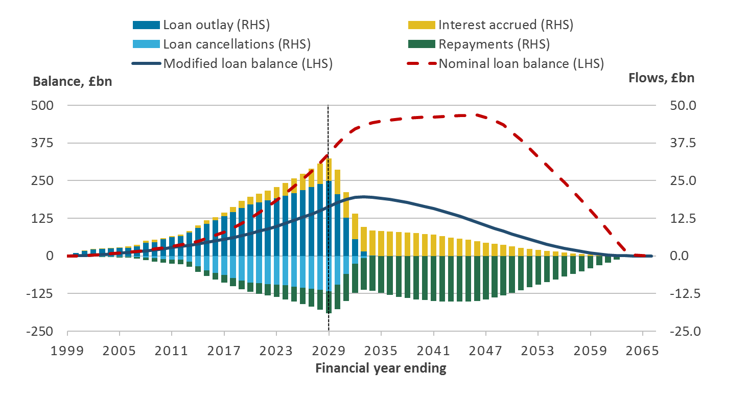
Figure 7: Under the partitioned loan-transfer approach, the loan balance is recorded net of amounts that are unlikely to be repaid
Population of student loans, UK, financial year ending 1999 to financial year ending 2066
Source: Office for National Statistics using Department for Education’s forecasts
Notes:
- Figures are provisional estimates. We have modelled at an individual level Plan 1 and Plan 2 student loans extended in England; an uplift is used to account for other types of loan in the UK.
- The final cohort of new students in the data consists of who receive the first part of their loans in FYE 2029.
Download this image Figure 7: Under the partitioned loan-transfer approach, the loan balance is recorded net of amounts that are unlikely to be repaid
.png (92.2 kB) .xlsx (42.9 kB)
Figure 7 plots the results. Transactions that increase the loan balance, such as outlay and interest, are shown above the horizontal axis. Those decreasing the balance – cancellation at inception and repayments – are shown below the axis.
We estimate that in FYE 2019, the Student Loans Company extended over £15.8 billion to students, both those who started their courses in the earlier years and to the cohort starting their studies in 2018. Of that amount, about £8.2 billion are deemed to be cancelled at inception and about £7.6 billion recorded as modified lending under the partitioned approach. The repayments, both for the loans extended in the previous years and during FYE 2019, stand at around £2.8 billion, of which almost £2.3 billion is accounted for by repayments on Plan 1 loans. The modified loan balance at year start is £66.9 billion, with a further £2.4 billion of modified interest accruing on it during the year.
These results should be contrasted with the estimates obtained under the conventional lending approach. The same outlay and repayment data result in a £107.7 billion opening nominal loan balance, with approximately £4.8 billion of nominal interest accruing during the year.
The difference is expected to be even greater in the subsequent years. In the final year for which outlay to new students is estimated, that is, FYE 2029, £23.9 billion of outlay are partitioned into £11.3 billion transfer (cancellation at inception) and £12.6 billion modified lending. The modified stock value at the beginning of the year is £164.0 billion, compared with £340.5 billion under the conventional lending approach. Since, at any point, the nominal interest accruing on nominal stock (under the conventional lending approach) is greater than repayments, the nominal stock on loans is ever-increasing (to a peak of £467.2 billion in the 2040s for students entering university before FYE 2029) and is ultimately cancelled at the end of the term date, assuming a closed system.
6.3. Impact on fiscal aggregates
In the previous sections, we described the results obtained using the new partitioned approach. At the point of implementation, however, the public sector finance (PSF) statistics were affected, not only by inclusion of the new estimates, but also by the removal of the old ones.
In this section, we use the versions of public sector net borrowing (PSNB) and public sector net debt (PSND) that include net borrowing of general government and public corporations but exclude publicly controlled commercial banks such as the Royal Bank of Scotland. In fiscal statistics, these series are known as “PSNB ex” and “PSND ex”.
In simple terms, when the new treatment was introduced, revenue from interest accruing on the entire nominal loan balance was replaced by interest on the proportion of loans that are likely to be repaid. In addition, debt cancellation at inception was recorded for the first time. Together with the impact from the loan book sales described in Section 5.5, the total PSNB impact of the transition was an increase of £12.4 billion in FYE 2019, the last complete financial year which preceded the implementation of the new partitioned treatment.
Table 3: Impacts of the student loan treatment change on public sector net borrowing excluding public sector banks (PSNB ex), financial year ending 1999 to financial year ending 2019
| UK, £billion | |||
|---|---|---|---|
| Financial year ending | PSNB ex under conventional loan treatment | Impact of treatment change | PSNB ex under partitioned treatment |
| 1999 | -1.1 | 0.0 | -1.1 |
| 2000 | -11.0 | 0.1 | -10.9 |
| 2001 | -16.1 | 0.2 | -15.9 |
| 2002 | 4.4 | 0.2 | 4.6 |
| 2003 | 32.1 | 0.2 | 32.3 |
| 2004 | 38.8 | 0.2 | 39.0 |
| 2005 | 46.1 | 0.3 | 46.4 |
| 2006 | 41.6 | 0.3 | 41.9 |
| 2007 | 38.0 | 0.4 | 38.4 |
| 2008 | 42.9 | 0.6 | 43.5 |
| 2009 | 113.5 | 0.8 | 114.3 |
| 2010 | 153.1 | 1.5 | 154.6 |
| 2011 | 136.5 | 1.2 | 137.7 |
| 2012 | 116.3 | 1.3 | 117.6 |
| 2013 | 120.3 | 2.2 | 122.5 |
| 2014 | 97.7 | 3.8 | 101.5 |
| 2015 | 89.9 | 5.4 | 95.3 |
| 2016 | 71.8 | 6.5 | 78.3 |
| 2017 | 44.9 | 7.5 | 52.4 |
| 2018 | 41.8 | 9.9 | 51.7 |
| 2019 | 23.5 | 12.4 | 35.9 |
| Source: Office for National Statistics using Department for Education's forecasts | |||
Download this table Table 3: Impacts of the student loan treatment change on public sector net borrowing excluding public sector banks (PSNB ex), financial year ending 1999 to financial year ending 2019
.xls (60.4 kB)The impacts in Table 3 differ from the earlier provisional estimates, such as those in the Office for Budget Responsibility’s (OBR’s) Economic and Fiscal Outlook: March 2019, and in the ONS articles published before September 2019. This is, in part, owing to improvements in the modelling methods, and in part because after the those publications were released, we concluded that additional expenditure should be recorded at the point of the loan book sales.
The change from the treatment of student loans as conventional loans to using the partitioned loan-transfer treatment has no effect on the contribution made by student loans to PSND. This is a narrow balance sheet measure that nets off government’s assets in cash and deposits from its liabilities in cash and deposits, bonds, and loans. As such, PSND does not account for the government’s stock of student loans, only the accumulation of cash transactions that have been made relating to student loans (outlays and repayments).
Public sector net financial liabilities (PSNFL) is a broader balance sheet measure that does consider the government’s student loan stock and was affected by the change in treatment: the nominal stock of loans was replaced by the modified loan balance in the calculation of PSNFL. The impact on PSNFL at the point of transition to the new treatment in September 2019 was an increase of £55.9 billion in FYE 2019.
Table 4: Impacts of the student loan treatment change on public sector net financial liabilities (PSNFL), financial year ending 1999 to financial year ending 2019
| UK, £billion | |||
|---|---|---|---|
| Financial year ending | PSNFL under conventional loan treatment | Impact of treatment change | PSNFL under partitioned treatment |
| 1999 | 314.5 | -0.2 | 314.3 |
| 2000 | 282.6 | 0.0 | 282.6 |
| 2001 | 287.0 | -0.1 | 286.9 |
| 2002 | 314.0 | -0.2 | 313.8 |
| 2003 | 366.1 | -0.6 | 365.5 |
| 2004 | 384.6 | -0.7 | 383.9 |
| 2005 | 428.6 | -1.1 | 427.5 |
| 2006 | 432.3 | -1.3 | 431.0 |
| 2007 | 457.8 | -0.9 | 456.9 |
| 2008 | 507.6 | -0.1 | 507.5 |
| 2009 | 707.5 | 1.0 | 708.5 |
| 2010 | 829.9 | 1.9 | 831.8 |
| 2011 | 935.9 | 2.8 | 938.7 |
| 2012 | 1067.5 | 4.3 | 1071.8 |
| 2013 | 1192.4 | 6.3 | 1198.7 |
| 2014 | 1271.0 | 10.5 | 1281.5 |
| 2015 | 1342.4 | 16.3 | 1358.7 |
| 2016 | 1417.8 | 22.9 | 1440.7 |
| 2017 | 1461.8 | 31.2 | 1493.0 |
| 2018 | 1424.9 | 39.8 | 1464.7 |
| 2019 | 1449.3 | 55.9 | 1505.2 |
| Source: Office for National Statistics using Department for Education's forecasts | |||
Download this table Table 4: Impacts of the student loan treatment change on public sector net financial liabilities (PSNFL), financial year ending 1999 to financial year ending 2019
.xls (47.6 kB)Notes for: Provisional results
- Owing to the timing of data processing by HM Revenue and Customs (HMRC) and the Student Loans Company (SLC), outturn data on outlay and direct repayments to SLC are available up to FYE 2018, but repayments made via HMRC and interest accruals are only available up to FYE 2017.
7. Conclusion
In September 2019, the public sector finance (PSF) statistics will saw a transition to a new treatment of student loans. The core idea behind the new approach is that for statistical purposes, income contingent instruments such as UK student loans should be treated as a combination of conventional lending and unrequited expenditure.
The partitioning is done so that the amount considered conventional lending can be fully repaid, with interest, by the end of the loan term. The amounts that exceed borrowers’ expected repayments areis recorded as expenditure at the point of loan extension.
The partitioning is therefore based on the forecasts of how much money the government will eventually get back. With such a lengthy forecast horizon, the estimates are sensitive to changes in assumptions, and there will inevitably be discrepancies between the forecasts and the outturn. It is also possible that the government may amend parameters associated with the repayment amounts, such as the repayment threshold, between loan extension and maturity.
To reflect these changes to expectations, we will be regularly updating loan stock values. Some of the updates, such as those caused by routine changes in economic forecasts or the discounting factor, will be incorporated into the data without affecting public sector net borrowing (PSNB). Others, such as policy changes leading to significantly different repayment expectations, will lead to recording of additional revenue or expenditure at the point of enactment, and so will have an impact on PSNB. Therefore, when we update the loan stock values to reflect changes in expectations, we will do so at a single point in time without making backwards revisions to PSNB.
The transition to the new treatment in September 2019 saw PSNB increasing by £12.4 billion, and PSNFL rising by £55.9 billion in the financial year ending (FYE) March 2019. These revisions differed slightly from the provisional estimates published before September 2019 for the following reasons:
- we extended the individual-level modelling to cover all types of student loan in the UK and performed further quality assurance of the data
- we analysed the pre-2012 student loan sales conducted by the government in 2017 and 2018, and concluded that under the new treatment, the sales increased PSNB by £1.5 billion in the FYE March 2019
8. Annex 1: Partitioning step by step
The main principles of the partitioned loan-transfer model can be expressed as equations. With a simplifying assumption that a loan is extended in a single instalment in financial year n, the following should hold for each student:
(4)
Over the lifetime of the loan:
(5)
Combining equations 4 and 5:
(6)
Equation 6 implies that estimating the lending and transfer components of the loan outlay requires working backwards from estimates of both the level of future repayments and the interest rates that will be applied (to the lending component) over the lifetime of the loan.
In practice, many borrowers, including those in the second or third year of their degree, would have taken out loans prior to the start of year n, and have an outstanding loan balance at the start of that financial year. If they subsequently take out further loans during or after year n, their repayments will be split to pay down both their new and outstanding balance. How the repayments should be divided is decided by valuing their new outlay at the same point in time as their existing balance (also at the beginning of the model year). The future outlay is discounted at the borrower’s interest rate.
For example, suppose that a borrower has a loan balance of £20,000 at the beginning of financial year ending (FYE) 2019 (either from previous courses or being mid-way through a course). They take out a final set of loans totalling £12,800 over FYE 2019. Their in-study interest rate is 6.22% in FYE 2019, and the loan is paid in instalments throughout the financial year, as described in Table 5. The value of the loan at the start of FYE 2019 is £12,496. As such, of any repayments they make, 61.5% of the repayment would go towards paying down their original balance, and 38.5% to paying down the loan they took out for FYE 2019.
Table 5: Illustrative example of splitting a borrower’s repayments between stock and future loans, for £12,800 loan for financial year ending (FYE) 2019 and £20,000 previous balance
| Components of loan | Nominal value (£) | Value at start of FYE 2019 (£) | Description | Repayment proportion (%) |
|---|---|---|---|---|
| Previous balance | 20,000 | 20,000 | Current value | 61.5 |
| End April 2018 payment | 5,808 | 5,778 | Value 1 months earlier | 17.8 |
| End September 2018 payment | 3,496 | 3,393 | Value 6 months earlier | 10.4 |
| End January 2019 payment | 3,496 | 3,325 | Value 10 months earlier | 10.2 |
| Total | 32,496 | 100.0 | ||
| Source: Office for National Statistics | ||||
| Notes: | ||||
| 1. Repayment proportions do not sum to 100% due to rounding. | ||||
Download this table Table 5: Illustrative example of splitting a borrower’s repayments between stock and future loans, for £12,800 loan for financial year ending (FYE) 2019 and £20,000 previous balance
.xls (60.4 kB)Then, taking into account that repayments may pay down loan balances from multiple courses, the transfer on forecast outlay and the total loan balance inclusive of previous loans can be calculated. The following describes the methodological steps involved in arriving at these estimates.
Step 1: Stock proportion (SP)
This is the proportion of repayments which will pay down loans taken out prior to the start of year n. The repayments (Rn) occurring in financial year (n) can be split into two values:
(7)
(8)
where RnStock is the component of repayments paying down loans taken out prior to year n and Rnfor is the component of repayments paying down loans that are forecast to be taken out in or after the model year.
Step 2: Cumulative repayments (CRfor) applied to forecast loans at the start of financial year n
This term takes into account the value of repayments made up to the start of financial year n by inflating them by the interest rate applied to the loan. Cumulative repayments from the previous year will have increased in value by an extra year of interest (Int) at the same rate as charged on the loan. This is a fixed rate for Plan 1 loans, and between the Retail Prices Index (RPI) and RPI plus 3 percentage points for Plan 2 loans.
New repayments (RNfor) made during the previous financial year are assumed to occur in the middle of the financial year, so increase in value by the equivalent of six months of interest to the start of the next financial year. Only those repayments not paying down loans taken out prior to the model year can pay off the forecast loans.
(9)
Step 3: Loan balance of forecast outlay at the start of financial year n based on repayments (RBalfor)
Working backwards from the end of the loan term to the start of financial year n, this is the balance, which would have been paid off with interest accruing on it.
(10)
Step 4: Loan balance at the start of financial year n based on outlay (OBaln)
Outlay (Outn) is provided over a financial year. It is assumed that three outlay payments will occur over the financial year: 1 month (Outn1), 6 months (Outn6) and 10 months (Outn10) into the financial year. Then, OBal is the loan balance based purely on outlay, and grows with interest. It does not take into account repayments.
(11)
(12)
Step 5: Lending proportion (Prop)
This is the expected proportion of forecast outlay paid back over the lifetime of the loan. The lending proportion is stable from Statutory Repayment Due Date (SRDD)2 to the end of the loan term, that is, once all outlay has been provided.
Cumulative repayments at SRDD represents any prepayments made before SRDD, inflated to their value at SRDD (as in Equation 9), while loan balance based on repayments represents the total amount repaid after SRDD, discounted to SRDD (as in Equation 10). Loan balance based on outlay represents the individual’s loan balance (excluding any prepayments) at SRDD (as in Equation 12).
(13)
Step 6: Transfer (T) and lending (L) during financial year n
The component of outlay classified as a transfer is the outlay that is not expected to be received back through repayments; lending is the component of the outlay that is expected to be received back. Transfer and lending can be calculated as follows respectively:
(14)
(15)
Step 7: Modified loan balance (MLB) at the start of financial year n
This is the balance of the lending component of the loan outlay in each financial year. It is equal to the modified loan balance at the start of the next financial year, deflated by one year’s worth of interest, increased by repayments occurring during this financial year (deflated by the interest they would otherwise accrue) and reduced by any outlay (and associated interest) that would be given out during that financial year.
An important point to make in relation to interest is that it accrues on the entire outstanding balance (not just on “principal” or the balance at the beginning of the first period) and is capitalised. As a result, while the relative timing matters, the balance does not depend on the partitioning mechanism applied to repayments.
Suppose that repayments go towards the principal first. At the end of the period, the original balance is reduced by the full value of the repayment, but this reduction is immediately offset by the capitalised interest that has accrued on the starting balance. Should the amount of the repayment exceed the amount of interest accrued in the same accounting period, it decreases the overall balance. This is calculated as follows:
(16)
Step 8: Modified interest (MInt) added to the modified loan balance during financial year n
Modified interest can be expressed as the difference between modified loan balances in the present and next financial year given repayments and lending during this financial year. This is calculated as follows:
(17)
Notes for: Annex 1: Partitioning step by step
- Borrowers are eligible to start repaying their loans in the April of the year after they graduated or left their course.
9. Annex 2: Impacts of forecast changes on a cohort of borrowers
9.1. Forecast change: revised economic expectations
In Section 5, we explained that economic forecasts are sensitive to changes in expectations. For this reason, it is useful to demonstrate how the estimates are likely to be changing over the course of the year without the interference of new policies or major economic events.
Most assumptions, such as earnings growth, inflation and economic growth are based on the Office for Budget Responsibility’s (OBR’s) macroeconomic projections. As an indicative example of the magnitude of the forecast changes we expect to make under the portioned loan-transfer approach. Figure 8 shows a transition from the assumptions based on the Economic and Fiscal Outlook: March 2019 to assumptions based on the Economic and Fiscal Outlook: October 2018.
The baseline model uses the latest OBR forecasts to maintain consistency with the other baseline estimates we present throughout this article. This example is representative of a routine change to assumptions that takes place as part of regular estimation updates. We will not usually update the forecast using an older set of assumptions in this way; however, this example is useful for demonstrating the size of revaluation of the loan stock that is required (as described in Section 5.4) when assumptions are routinely changed. While both forecasts have been produced at the time of the lasting Brexit uncertainty, there is no step change in expectations between them.
Figure 8: Under the partitioned loan-transfer approach, the loan balance is revalued when macroeconomic assumptions are changed
Illustrative example based on the 2018 to 2019 cohort of students, England, financial year ending 2019 to financial year ending 2056

Source: Office for National Statistics using Department for Education's forecasts
Notes:
- By cohort we understand a group of students that receive the first part of their student loans in a given academic year.
- Macroeconomic assumptions are revised on 1 April 2019.
Download this image Figure 8: Under the partitioned loan-transfer approach, the loan balance is revalued when macroeconomic assumptions are changed
.png (35.3 kB) .xlsx (39.1 kB)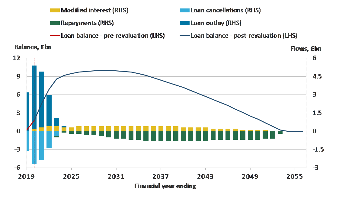
Prior to 1 April 2019, March 2019 macroeconomic assumptions were in place. Thereafter, the results are produced using the October 2018 assumptions. Joining the two time series requires a downward revaluation of loan stock of £25 million, or around 1.3% of the £1.8 billion stock valued using the older set of assumptions.
9.2. Forecast change: interest rate change
Government actions are also likely to alter the economic value of the loan stock. One such hypothetical action is a change in the interest rate base. Since their introduction, interest rates on Plan 2 loans have been linked to the Retail Prices Index (RPI).
Depending on the borrower’s earnings, the annual rate varies in the interval between RPI (faced mainly by low-earners) and RPI plus 3 percentage points (faced by borrowers at the higher end of the income distribution). It is conceivable that government might choose to rebase the existing loans onto the Consumer Prices Index-based (CPI-based) interest rate scale. The rebase will have varied effects across the borrowers’ income distribution. The consequence of this is that the statistical aggregates will be impacted by two effects acting in the opposite directions.
The high-earners, or those who are likely to repay their loan and interest accrued on it in full, will see a reduction in interest rates, and so a reduction in the amounts they repay over the loan term. For these borrowers, there is no transfer at inception:
(18)
Rearranging for the existing borrowers where there is no new lending and so no new partitioning, we replace Lendingn with the accumulated past lending at time n + x or the discounted value of the borrower’s loan balance MLBn+x. This is calculated as follows:
(19)
Over time, government revenue will be reduced by the amount of interest foregone. However, because the reduction in repayments is driven exclusively by a drop in interest rates, there is no impact on the amount borrowed, and so on the value of the loan balance. That would of course apply to new borrowers whose income is predicted to be high too.
The second and arguably the main effect is that borrowers on lower incomes will see less interest added to their nominal (non-partitioned) balance. They may not be able to repay the balance in full, so their total repayments over the loan term may remain unaffected. Rearranging the same equation for existing borrowers again, we can show the impact on their loan value as follows:
(20)
Perhaps counter-intuitively, the value of the loan increases. As we discussed in Section 5.4, this effect is merely reflecting the fact that the lower the interest, the higher the “principal” affordable to the borrowers.
In combination, the two effects tend to increase the value of the loan book initially but subsequently reduce government revenue from interest accruing on the loan balance.
Figure 9: Under the partitioned loan-transfer approach, the loan balance is revalued when the interest rates change
Illustrative example based on the 2018 to 2019 cohort of students, England, financial year ending 2019 to financial year ending 2056
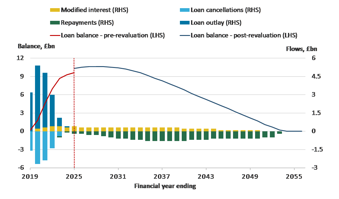
Source: Office for National Statistics using Department for Education's forecasts
Notes:
- By cohort we understand a group of students that receive the first part of their student loans in a given academic year.
- The base used to calculate interest rates is changed from the Retail Prices Index (RPI) to the Consumer Prices Index (CPI) on 1 April 2024.
Download this image Figure 9: Under the partitioned loan-transfer approach, the loan balance is revalued when the interest rates change
.png (36.0 kB) .xlsx (39.3 kB)
Figure 9 puts this into practice using our estimates for the cohort of students starting in the academic year beginning 2018, rebasing the interest rates from RPI to CPI on 1 April 2024. At that date, we estimate that the modified loan balance will stand at £9.6 billion.
In that following year, the interest accruing on the loan stock will remain virtually unchanged by the policy change, at £0.4 billion – a decrease in the interest rate will be offset by an increase in lending. This is a temporary effect caused by the Plan 2 loan system still being in its relative infancy; as the system matures, interest revenues will drop relative to a baseline case. When the reform is enacted, a revaluation needs to be recorded to reflect an upward change in value of the cohort's loan stock, amounting to £0.7 billion (7.3% of the loan stock as valued before the policy change).
9.3. Forecast change: an example of major higher education funding reform
Finally, we consider a larger change package that alters multiple conditions of the existing student loans in the single cohort. The effects of this reform may differ from a reform that only alters loan conditions for future borrowers in the population. We have chosen to model a decrease in the repayment threshold1 alongside a rebase of the interest rates from RPI to CPI, both policies being enacted on 1 April 2024.
The former reform component, a threshold decrease, reduces the total amount of repayments that the government can expect to collect, thereby increasing the transfer element within outlay. This is calculated as follows:
(21)
In relation to existing borrowers at time n + x, it similarly decreases the value of the loan balance:
(22)
As we described in Section 9.2, the impact of a reduction in interest rates is to increase the value of the loan balance at the point of policy enactment, through a change in the rate at which future repayments are discounted. In this sense, the interest rate reduction acts in the same direction as the lower repayment threshold when the policy package is implemented.
This is confirmed by modelling: if the reform package is introduced on 1 April 2024, the loan stock value increases by £1.3 billion (13.5%) thanks to a combination of higher expected repayments from the repayment threshold decrease, and a reduction in the discount rate. In contrast to the scenario presented in Section 9.2, the modified loan balance is significantly affected by the expected change in future repayments. Although some of the increase in the loan stock value is because of a decrease in the discount rate, it is impractical to separate the two effects of the policy changes, so a capital transfer of £1.3 billion (the same value as the loan balance increase) needs to be recorded.
Figure 10: Under the partitioned loan-transfer approach, the loan balance is revalued and a transfer is recorded when the stock value is significantly affected by the change in expected future repayments
Illustrative example based on the 2018 to 2019 cohort of students, England, financial year ending 2019 to financial year ending 2056
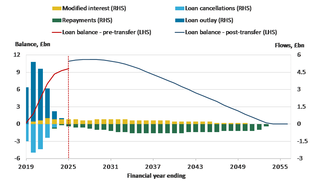
Source: Office for National Statistics using Department for Education's forecasts
Notes:
- By cohort we understand a group of students that receive the first part of their student loans in a given academic year.
- Policy changes are implemented on 1 April 2024.
Download this image Figure 10: Under the partitioned loan-transfer approach, the loan balance is revalued and a transfer is recorded when the stock value is significantly affected by the change in expected future repayments
.png (37.4 kB) .xlsx (39.2 kB)
Notes for: Annex 2: Impacts of forecast changes on a cohort of borrowers
The change modelled was a decrease in both the lower and upper repayment thresholds by £2,000, increasing annually by forecast average earnings thereafter.
There is a feedback loop between lending and modified interest. A decrease in lending would reduce the loan balance and thus the interest accruing on it. Equation 21 is therefore only showing the direct initial impact.
10. Annex 3: Alternative valuations of future repayments
We explained in Section 4.1 that for national accounting purposes, the partitioned loan-transfer methodology estimates the statistical value of future student loan repayments based on the loan balance, principle and interest expected to be fully repaid before the loans are cancelled. Valuations of expected future forecast repayments differ depending on their uses by different government bodies, and the various methodologies used.
Table 6 provides a descriptive overview of the differences between three valuations of future repayments:
- the statistical value used for the UK National Accounts
- the accounting value used for the Resource Accounting and Budgeting (RAB) cost in the Department for Education’s financial statements
- the valuation used by the government when assessing the value for money of a student loan sale
| Statistical value, used by the Office for National Statistics | Accounting value, used by the Department for Education | UK Government's loan sale value for money assessment | |
|---|---|---|---|
| Forecast model and coverage | Model for the entire loan book with sample limited to loans being sold | Model for the entire loan book with sample limited to loans being sold | Model developed specifically for the loans being sold |
| Discounting approach | Discounting uses rate based on individual borrower interest rates and future cashflow projections to estimate loan balance that will be fully repaid with interest | Discounting uses a rate of retail price index plus 0.7%, consistent with the Government Financial Reporting Manual1 | Discounting uses a rate comprising a hurdle rate and risk premium specific to the asset being valued, per government-wide asset sales guidance in the Green Book2 |
| No explicit consideration of risk related to future asset cashflows | No explicit consideration of risk related to future asset cashflows | Compensation for the risk of future asset cashflows is explicitly considered in a manner comparable to market valuation theory and practice | |
| Intended use | Estimating a statistical value for what loan balance will be if fully repaid with interest at a point of time | Setting out a value for a long-dated asset in a manner consistent with HM Treasury’s overall accounting guidelines for all government financial assets | Assessing a present value for a loan asset given alternative uses of cash plus compensation for risk specific to that asset |