Table of contents
- Main points
- Statistician’s comment
- Things you need to know about this release
- Median household disposable income £1,600 higher than pre-downturn level
- Median disposable income of richest fifth recovers to pre-downturn levels for first time
- How much do cash benefits and direct taxes reduce income inequality?
- Gradual decline in income inequality over the last decade
- How do incomes for retired and non-retired households compare?
- Inequality rose for retired households but fell for non-retired households in recent years
- Policy context: changes to taxes and benefits during the financial year ending 2017
- Economic context
- What has changed in this publication?
- Upcoming changes to this bulletin
- Users and uses of these statistics
- Links to related statistics
- Quality and methodology
1. Main points
- Based on the Office for National Statistics’s (ONS’s) Living Costs and Food Survey, the UK median disposable household income was £27,300 in the financial year ending (FYE) 2017, up 2.3% on the previous year (after accounting for inflation and household composition).
- The latest estimate of UK median disposable household income is very similar to the nowcast estimate of £27,200 for FYE 2017, published in July 2017.
- Growth in median disposable income for the richest fifth of households has lagged behind households in the rest of the income distribution in recent years, but has now recovered to the levels seen before the start of the economic downturn, taking into account inflation and changes in household composition.
- There has been a small decline in income inequality in the last 10 years, although inequality in FYE 2017 (based on the Living Costs and Food Survey) at 32.2% is broadly unchanged from FYE 2016 (31.6%).
- Between FYE 2016 and FYE 2017, both retired and non-retired households have seen increases in their median disposable incomes, though the growth has been larger for non-retired households (3.5%) than for retired households (1.2%).
2. Statistician’s comment
Commenting on today's figures on household income, Head of Well-being and Inequalities Glenn Everett said:
"Households have more disposable income than at any time previously. However, compared with their pre-downturn levels the incomes of the poorest households have risen nearly two thousand pounds but the incomes of the richest are only now slightly higher. Overall, income inequality has slowly fallen over the last decade."
Back to table of contents3. Things you need to know about this release
Sources of income estimates
This release provides headline estimates from the effects of taxes and benefits on household income (ETB) and has been designed to provide more timely figures of main indicators. ETB data are from the Office for National Statistics’s (ONS’s) Living Costs and Food Survey (LCF), a voluntary sample survey of around 5,000 private households in the UK.
An important strength of the ETB data is that comparable estimates are available back to 1977, allowing analysis of long-term trends, and expenditure data are also available for the sampled households. This release also currently provides the earliest survey-based analysis of the household income distribution available each year, allowing people insight into the evolution of living standards as early as possible.
However, as with all survey-based sources, the data are subject to some limitations. The LCF is known to suffer from under-reporting at the top and bottom of the income distribution as well as non-response error (see The effects of taxes and benefits upon household income Quality and Methodology Information report for further details of the sources of error).
The Department for Work and Pensions (DWP) also produces an analysis of the UK income distribution in its annual Households below average income (HBAI) publication, using data from its Family Resources Survey (FRS). While the FRS is subject to the same limitations as other survey sources, it benefits from a larger sample size (approximately 19,000 households) than the LCF and, as such, will have a higher level of precision than ETB estimates. In addition, HBAI includes an adjustment for “very rich” households to correct for the under-reporting using data from HM Revenue and Customs’s (HMRC’s) Survey of Personal Incomes (SPI). These differences make HBAI a better source for looking at income-based analysis that does not need a very long time series (the FRS data are available from financial year ending (FYE) 1995) and when looking at smaller sub-groups of the population, particularly at the upper end of the income distribution.
In order to address some of the limitations with the current ETB estimates, ONS is currently working on transforming its data on the distribution of household finances. The first part of this work has concentrated on combining the samples from the LCF and another of ONS’s household surveys, the Survey on Living Conditions (SLC) and harmonising the income collection in these questionnaires so that these estimates from FYE 2018 onwards will benefit from a larger sample size of around 17,000 households.
In addition, ONS is working towards linking data from administrative and other non-survey sources, including HMRC Real Time Information (RTI) and DWP benefits data. Although these other sources also have their own limitations, by using them together with surveys we should be able to produce better data on household income. For further information on other sources of income and earnings data, including the appropriate uses of and limitations of each data source see A guide to sources of data on earnings and income.
What is average household income?
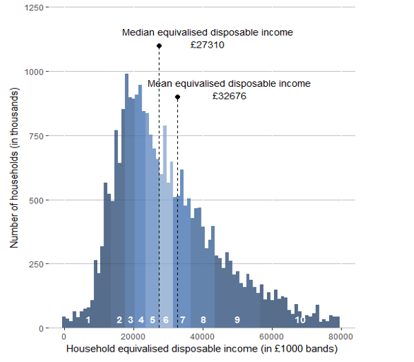
This bulletin looks at two main measures of average household income, the mean and the median. Figure 1 shows the distribution of equivalised disposable income for FYE 2017, clearly indicating the skewness of the distribution; the mean income level (£32,700) is greater than the median (£27,300). The greatest number of households (mode) falls into the £17,000 to £18,000 bracket, which is in the third decile of the distribution.
Figure 1: Distribution of UK household disposable income, financial year ending 2017
Source: Office for National Statistics
Notes:
- No expenditure on housing costs (apart from Council Tax) is deducted from disposable income in this release. HBAI estimates are available before and after housing costs – see the Households below average income (HBAI) publication for further details.
Download this image Figure 1: Distribution of UK household disposable income, financial year ending 2017
.png (62.5 kB) .xls (30.2 kB)
The mean simply divides the total income of households by the number of households. A limitation of using the mean is that it can be influenced by just a few households with very high incomes and therefore does not necessarily reflect the standard of living of the “typical” household. However, when breaking down changes in income and direct taxes by income decile or types of households, the mean allows for these changes to be analysed in an additive way.
Many researchers argue that growth in median household incomes provides a better measure of how people’s well-being has changed over time. The median household income is the income of what would be the middle household, if all households in the UK were sorted in a list from poorest to richest. As it represents the middle of the income distribution, the median household income provides a good indication of the standard of living of the “typical” household in terms of income.
What is disposable income?
Disposable income is arguably the most widely used household income measure. Disposable income is the amount of money that households have available for spending and saving after direct taxes (such as Income Tax, National Insurance and Council Tax) have been accounted for. It includes earnings from employment, private pensions and investments as well as cash benefits provided by the state.
Figure 2: Stages in the redistribution of income

Source: Office for National Statistics
Download this image Figure 2: Stages in the redistribution of income
.png (44.6 kB)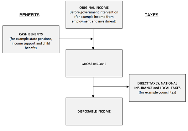
Comparisons over time
This bulletin looks at how main estimates of household incomes and inequality have changed over time. In order to make robust comparisons historic data have been adjusted for the effects of inflation and are equivalised to take account of changes in household composition. More information on the details of these adjustments can be found in the Quality and methodology section of this bulletin.
Estimates in this release are not based on a longitudinal data source so the composition of households differs between periods of time. When growth rates are quoted, they compare the average for a group of households in one period to the average for a different set of households in the next period.
Statistical significance
Statistical significance indicates whether a reported change is likely to have occurred by chance. Any change that has been described as significant is significant at the 95% level. This means that the probability that the difference occurred by chance is low (1 in 20 or lower).
Back to table of contents4. Median household disposable income £1,600 higher than pre-downturn level
The median equivalised household disposable income in the UK was £27,300 in the financial year ending (FYE) 2017. After taking account of inflation and changes in household structures over time, the median disposable income has increased by £600 (or 2.3%) since FYE 2016 and is £1,600 higher than the pre-economic downturn level observed in FYE 2008. The year-on-year growth rate is broadly in line with the average growth rate per year for the past 40 years with median household income growing from £12,500 at an average rate of 2.1% per year between 1977 and FYE 2017.
Figure 3: Growth of median (and mean) household income and gross domestic product per head
Source: Office for National Statistics
Notes:
- GDP per head has been adjusted for inflation using National Accounts methods; the mean and median time series have been adjusted for inflation using the consumer prices index including owner-occupiers’ housing costs (CPIH).
- Up until 1993, calendar year data are plotted against Quarter 3. From financial year ending 1995, data are plotted against Quarter 4.
Download this chart Figure 3: Growth of median (and mean) household income and gross domestic product per head
Image .csv .xlsFigure 3 shows the growth of gross domestic product (GDP) per head over the same timeframe. Growth in median household income closely mirrors growth in GDP per head for much of this time, rising during periods of economic growth and falling during or immediately after downturns.
The effect of the economic downturn on median household incomes was delayed relative to the fall in GDP per head. Between FYE 2008 and FYE 2010, GDP per head fell by 6.5%, while median disposable income changed little. However, between FYE 2010 and FYE 2013, GDP per head grew by 2.6%, while median household income decreased by 4.5%. Since FYE 2013, UK median household income has grown at a faster rate than GDP per head (11.6% and 6.6% respectively). (See the section ‘Economic context’ for further information.)
Preliminary estimates of main indicators such as median equivalised disposable income were released as Experimental Statistics in the bulletin Nowcasting household income in the UK: financial year ending 2017 in July 2017. These preliminary estimates made use of “nowcasting” techniques in order to produce figures before full survey-based estimates are available. The preliminary estimate of median disposable income for FYE 2017 was £27,200 compared with a final estimate of £27,300.
Back to table of contents5. Median disposable income of richest fifth recovers to pre-downturn levels for first time
The relative growth of median income by quintile since before the economic downturn in the financial year ending (FYE) 2008 is shown in Figure 4, after accounting for inflation and household structure.
While the average incomes of those in the bottom fifth of the population were consistently above their FYE 2008 level throughout this time, the income of the top fifth of the population only recovered to these levels for the first time in FYE 2017. Reflecting this, while the average income of the poorest fifth has risen by £1,800 (or 15.0%) since FYE 2008, that of the richest fifth is now at a broadly similar level, an increase of only £200 over this time period, which equates to an increase of less than 0.5%.
Figure 4: Growth in median equivalised household disposable income by quintile group, financial year ending 2008 to financial year ending 2017
Source: Office for National Statistics
Notes:
- Households are ranked by their equivalised disposable incomes, using the modified OECD scale.
- Growth is reported in real terms, that is estimates for earlier years have been adjusted to take account of inflation.
Download this chart Figure 4: Growth in median equivalised household disposable income by quintile group, financial year ending 2008 to financial year ending 2017
Image .csv .xlsThe increases in median income across the distribution are due mainly to an increase in the average income from employment, reflecting increases in both the wages and employment levels of people living in these households.
Back to table of contents6. How much do cash benefits and direct taxes reduce income inequality?
This section looks at the sources of earnings, benefits and taxes that make up the overall income measures and therefore the measurement of average household income used is the mean; the mean allows for changes in the components of disposable income to be analysed in an additive way. For more information on the different measures of average household income see the ‘Things you need to know about this release’ section.
Overall, direct taxes and cash benefits lead to income being shared more equally between households (Figure 5). In the financial year ending (FYE) 2017, before direct taxes and cash benefits, the richest fifth (those in the top income quintile group) had an average original income of £88,800 per year, compared with £7,400 for the poorest fifth – a ratio of 12 to 1. (Original income includes earnings, private pensions1, and investments.) This ratio is unchanged since FYE 2016, indicating that inequality of original income has stayed the same, according to this measure.
Figure 5: Original, gross and disposable income by quintile group, all households, financial year ending 2017
Source: Office for National Statistics
Notes:
- Households are ranked by their equivalised disposable incomes, using the modified OECD scale.
Download this chart Figure 5: Original, gross and disposable income by quintile group, all households, financial year ending 2017
Image .csv .xlsEffect of cash benefits
In contrast to original income, the amount received from cash benefits such as tax credits, Housing Benefit and Income Support tends to be higher for poorer households than for richer households. The highest average amount of cash benefits were received by households in the second quintile group, £9,100 per year compared with £8,000 for households in the bottom group, a trend that has remained unchanged since FYE 1996. This is largely because the State Pension, which in this analysis is classified as a cash benefit, makes up the largest proportion of the total cash benefits received by households and there are, on average, more retired people in households in the second quintile group than the bottom group.
The distribution of cash benefits between richer and poorer households has the effect of reducing inequality of income. After cash benefits were taken into account, the richest fifth had an average income that was roughly six times the poorest fifth (gross incomes of £92,000 per year compared with £15,300, respectively), a proportion that is unchanged on the previous year.
Looking at individual cash benefits, in FYE 2017, the average combined amount of contribution-based and income-based Jobseeker’s Allowance (JSA) received by the bottom two-fifths of households decreased compared with FYE 2016 (Reference Table 2 in the Household disposable income and inequality dataset). This is due largely to fewer households receiving this benefit. This is consistent with a fall in unemployment between these years, as well as the ongoing implementation of the Universal Credit (UC) system which, by April 2017, had been rolled out to almost half a million claimants2. The Claimant Commitment, which outlines specific actions that claimants of UC and JSA must carry out in order to receive benefits, may also have affected the number of recipients of these benefits. For those recipients still in receipt of JSA, in common with other working age benefits, rates were frozen in FYE 2017.
The phasing out of Incapacity Benefit, Severe Disablement Allowance and Income Support paid because of illness or disability and transfer of recipients to Employment and Support Allowance (ESA) has seen average amounts received from the former benefits continue to fall in FYE 2017. The roll-out of Personal Independence Payment (PIP), which is replacing Disability Living Allowance (DLA) for adults aged under 65, also continued in FYE 2017.
Effect of direct taxes
On average, households paid £8,400 per year in direct taxes, equivalent to 19.2% of their gross income. Richer households pay both higher amounts of direct tax and higher proportions of their income in direct taxes (Income Tax, National Insurance, and Council Tax and Northern Ireland rates). As a result, direct taxes also reduce inequality of income.
The richest fifth of households paid on average £21,400 in direct taxes in FYE 2017, the vast majority of which (almost 70%) was Income Tax. This corresponds to 23.2% of their gross income, broadly unchanged from other recent years.
The average direct tax bill for the poorest fifth was £1,900, of which the largest component, over half, was Council Tax or Northern Ireland rates. This was equivalent to 12.7% of gross household income for this group, slightly higher than in FYE 2016 (11%).
The richest fifth of households had disposable incomes that were around five times that of the poorest fifth (£65,500 and £12,700 per year, respectively), a similar ratio to FYE 2016.
Figure 6 shows the relative contributions of the individual components of disposable income, to its overall growth in FYE 2017 for the different quintiles. The fourth quintile experienced the highest growth in mean disposable income, driven by an increase in income from employment. The poorest fifth experienced the lowest overall growth due to lower increases in income from employment and an increase in the average direct tax bill previously described.
Figure 6: Contribution to growth in mean disposable income by quintile group, financial year ending 2017
Source: Office for National Statistics
Notes:
- Households are ranked by their equivalised disposable incomes, using the modified OECD scale.
- Growth is reported in real terms, that is estimates for financial year ending 2016 have been adjusted to take account of inflation.
- Positive contributions indicate the data contribute more to income growth than the previous period. Negative contributions indicate the data reduce growth more than the previous period.
Download this chart Figure 6: Contribution to growth in mean disposable income by quintile group, financial year ending 2017
Image .csv .xlsIndirect taxes and benefits in-kind
Indirect taxes on expenditure (such as VAT and fuel and alcohol duties) and benefits in-kind provided by the state (such as education services and the NHS) also play a significant role in the redistribution of income.
The full Effects of taxes and benefits on household income, financial year ending 2017 statistical bulletin, to be released in summer 2018, will provide further analysis of household income including the effect of both of these.
Notes for: How much do cash benefits and direct taxes reduce income inequality?
- Private pensions include all non-state pensions whether occupational or personal.
- Data downloaded from DWP’s Stat-Xplore tool in October 2017.
7. Gradual decline in income inequality over the last decade
The Gini coefficient is a commonly-used measure of income inequality. Gini coefficients can vary between 0 and 100 and the lower the value, the more equally household income is distributed. Figure 7 shows the effects of cash benefits and taxes on reducing inequality, as measured by the Gini. Before taxes and benefits, inequality of original income was 48.9% in financial year ending (FYE) 2017. After taking account of cash benefits, inequality of gross income fell to 35.4%, with a further reduction to 32.2% for disposable income (after the effects of direct taxes are taken into account).
Figure 7: Gini coefficients for original, gross and disposable income using the Living Costs and Food Survey, financial year ending 2008 to financial year ending 2017
Source: Office for National Statistics
Download this chart Figure 7: Gini coefficients for original, gross and disposable income using the Living Costs and Food Survey, financial year ending 2008 to financial year ending 2017
Image .csv .xlsWhen looking at the change in inequality over the last 10 years, income inequality, as measured by the Gini coefficient, has shown a downward trend across all three measures of income. There has been no statistically significant change in the Gini for any of the income measures in the last year.
As noted in the section ‘Sources of income estimates’, the Households below average income (HBAI) statistics produced by the Department for Work and Pensions provide an alternative source of data on household incomes and inequality. Figure 8 shows the Gini coefficient for disposable income from HBAI (before housing costs) and the same statistic for disposable income from the effects of taxes and benefits (ETB) dataset. Both series are rounded to the nearest 0.1 percentage point for comparability.
Prior to FYE 2016, the two series showed a similar picture, with a small fall in inequality compared with FYE 2008. In FYE 2016, the two series diverged with a small rise in the Gini reported by HBAI and a small fall in the figure from the ETB data. The larger sample size and adjustment for high earners applied to HBAI mean that it is likely to be a stronger data source for these purposes. Nonetheless, over this period, the broad picture painted by both sources is of a small fall in inequality.
Figure 8: Gini coefficients for disposable income from effects of taxes and benefits and households below average income (before housing costs)
Financial year ending 2008 to financial year ending 2017
Source: Office for National Statistics
Notes:
- HBAI estimates for financial year ending 2017 were not yet available at the time of publication.
Download this chart Figure 8: Gini coefficients for disposable income from effects of taxes and benefits and households below average income (before housing costs)
Image .csv .xls8. How do incomes for retired and non-retired households compare?
Retired households are those where the income of retired household members accounts for the majority of the total gross household income (see the Glossary in the ‘Quality and methodology’ section for the definition of a retired person). Retired households have different income and expenditure patterns to their non-retired counterparts.
Figure 9 compares growth in the median equivalised disposable income of retired and non-retired households with all households. While the income of retired households remains considerably lower than that of non-retired households, retired households have seen faster income growth over the period covered. In 1977, after adjusting for inflation, the median income of retired households was £7,900 while the figure for non-retired households was £14,100. By the financial year ending (FYE) 2017, the income of retired households was 2.8 times higher at £22,300 while the income of non-retired households had only just over doubled to £29,900.
Figure 9: Median equivalised disposable household income by household type, financial year ending 2017
Source: Office for National Statistics
Notes:
- Estimates have been adjusted to take account of inflation.
Download this chart Figure 9: Median equivalised disposable household income by household type, financial year ending 2017
Image .csv .xlsThe pattern of change since the start of the economic downturn has also been very different for retired and non-retired households (Figure 10). Between FYE 2008 and FYE 2017, although incomes of non-retired households have remained higher than retired households, the median income of retired households increased by 14.3%. In contrast, the median income of non-retired households was consistently lower than its FYE 2008 level throughout this period until FYE 2017 when it exceeded it for the first time. As a result the median income of non-retired households increased only 2.3% between FYE 2008 and FYE 2017.
Since FYE 2013, retired and non-retired households have seen steady growth in their respective disposable income levels, though in the latest period, the growth has been larger for non-retired households (3.5%) than for retired households (1.2%).
The growth in the incomes of retired households since FYE 2008 has been driven by a number of factors. One is a rise in both the amounts received and the number of households reporting receipts from private pensions or annuities. (Private pensions include all non-state pensions whether occupational or personal.) Another is an increase in average income from the State Pension, due in part to the effect of the "triple lock"1.The fall in average disposable income for non-retired households after the economic downturn largely reflected a fall in income from employment (including self-employment).
Figure 10: Growth in median equivalised disposable household income by household type, financial year ending 2008 to financial year ending 2017
Source: Office for National Statistics
Notes:
- Growth is reported in real terms, that is estimates for earlier years have been adjusted to take account of inflation.
Download this chart Figure 10: Growth in median equivalised disposable household income by household type, financial year ending 2008 to financial year ending 2017
Image .csv .xlsFigure 11 shows how the sources of retired households’ incomes have changed over time. As we are looking at components of income, in this case, the average used is the mean.
Overall, the proportion of retired households’ average income coming from cash benefits (including the State Pension) fell from 64.7% in 1977 to the current level of 45.9%. This does not reflect a reduction in average amounts received but instead has been due mainly to the growth in the percentage of retired households receiving income from private pensions, which rose from 44.5% in 1977 to 82.1% in FYE 2017, and an increase in income from these pensions. In 1977, the average income received by retired households from private pensions was £1,600, accounting for 18% of the gross income of this group. By FYE 2017, the average income received by retired households from private pensions increased to £11,400, or 44.3%, of their gross income.
The State Pension was the second largest source of income for retired households in FYE 2017 and was the second largest source of growth, almost doubling from an average of £4,800 in 1977 to £9,500 in FYE 2017.
Figure 11: Percentage composition of mean gross income of retired households, financial year ending 2017
Source: Office for National Statistics
Download this chart Figure 11: Percentage composition of mean gross income of retired households, financial year ending 2017
Image .csv .xls9. Inequality rose for retired households but fell for non-retired households in recent years
As with previous sections the Gini coefficient is used as a measure of inequality in the distribution of household income, which can vary between 0 and 100 (the lower the value, the more equally household income is distributed).
Taxes and benefits have a particularly significant redistributive effect on the income of retired households, meaning that disposable income inequality is much lower for retired households than for non-retired households. Cash benefits play by far the largest part in bringing about this reduction, due principally to the State Pension. As a result, retired households’ Gini coefficient for disposable income was 28.0% in the financial year ending (FYE) 2017, compared with 32.5% for non-retired households (Figure 12).
Inequality of disposable income for both retired and non-retired households has followed a similar trend to that for all households, increasing during the 1980s. Since then the broad trend has been downwards, though income inequality levels remain above those seen in the late 1970s and early 1980s.
In recent years, there is evidence of an increase in inequality for retired households. Compared with the most recent low point, in FYE 2010, the Gini coefficient for disposable income amongst retired households has increased significantly by 3.7 percentage points. This in part reflects a growing gap between retired households in receipt of income from private pensions and those without private pensions (see What has happened to the income of retired households in the UK over the past 40 years?).
There has been more year-on-year variation in the Gini coefficients for retired households than for the overall population, though this is primarily a consequence of the smaller sample size on which these estimates are based.
Figure 12: Gini coefficients for disposable income by household type, 1977 to financial year ending 2017
Source: Office for National Statistics
Notes:
1.Estimates have been adjusted to take account of inflation.
Download this chart Figure 12: Gini coefficients for disposable income by household type, 1977 to financial year ending 2017
Image .csv .xls10. Policy context: changes to taxes and benefits during the financial year ending 2017
This section provides information and analysis on both the main changes to taxes and benefits in the financial year ending (FYE) 2017 and the wider economic trends over this period.
Some of the main tax and benefit changes occurring during FYE 2017 included the following.
National Minimum Wage and National Living Wage
In April 2016 a new National Living Wage of £7.20 per hour was introduced for employees aged 25 and over. Workers under the age of 25 years continue to get the National Minimum Wage, which increased from October 2016.
Analysis of the distribution of earnings across the UK using the Annual Survey of Hours and Earnings (ASHE) data 2016 and the Annual Survey of Hours and Earnings: 2017 provisional and 2016 revised results show the influence of the National Living Wage on earnings growth between 2015 and 2017. These tend to show that the largest percentage changes in earnings are experienced by those in the lower percentiles of the individual earnings distribution, see Figure 5 of the latter release.
Benefit freeze
Certain working-age benefits will be frozen at FYE 2016 cash values from FYE 2017 to FYE 2020. Benefits excluded from the freeze are: Disability Living Allowance; Personal Independence Payment; Employment and Support Allowance Support Group component; Carer benefits; Pension benefits; Maternity Allowance; Statutory Sick Pay; Statutory Maternity Pay; Statutory Paternity Pay; Statutory Shared Parental Pay; and Statutory Adoption Pay.
Benefit cap
A benefit cap in place in England, Scotland and Wales restricts the amount of certain benefits that a working-age household can receive. Any household receiving more than the cap has their Housing Benefit reduced to bring them back within the limit. This benefit cap was introduced in Northern Ireland from 31 May 2016 with a “Welfare Supplementary Payment” paid to any households with children in who have their Housing Benefit reduced due to the cap.
From 7 November 2016, the benefit cap was reduced from £26,000 to £23,000 for households living in London and to £20,000 for those outside London.
Those in receipt of Guardian's Allowance, Carer's Allowance and the carer's element of Universal Credit are exempt from the benefit cap.
Housing Benefit
From May 2016 in England, Scotland and Wales, the family premium included in Housing Benefit (£17.45 per month) was removed for families making a new claim for Housing Benefit. The allowed period for Housing Benefit backdating also decreased from six months to four weeks. This was applied in Northern Ireland from 5 September 2016.
Universal Credit
During FYE 2017 the roll-out of Universal Credit continued.
In FYE 2016, the childcare costs element of Universal Credit paid 70% of registered childcare costs up to a monthly limit of £532.29 a month for one child or £912.50 for two or more children. From 11 April 2016, this increased to 85% of childcare costs up to a monthly limit of £646.35 for one child or £1,108.04 for two or more children.
From April 2016, Universal Credit work allowances reduced to £4,764 for those without housing costs, £2,304 for those with housing costs, and the allowance was removed altogether for non-disabled claimants without children.
From November 2016, Universal Credit is a qualifying benefit for the Healthy Start Food Vouchers scheme.
Tax Credits
From April 2016, the Tax Credit income rise disregard, which is the limit household income can increase in a tax year before it impacts the calculation of entitlement for that year, decreased from £5,000 to £2,500. The rate at which Tax Credit awards are reduced (known as the taper rate) increased from 41% to 48%.
Income Tax
In April 2016, the tax-free personal allowance, which is the amount you can earn before paying any Income Tax, increased from £10,600 to £11,000. The higher rate (40%) tax threshold increased from £42,385 to £43,000. The age-related personal allowance came to an end in FYE 2017.
Income Tax: abolition of the £8,500 threshold for benefits in kind
From April 2016, the £8,500 threshold that determines whether employees pay Income Tax on all of their benefits in kind (for example, company car) and expenses is abolished. Employers will have additional National Insurance contributions to pay on the benefits in kind and certain expenses provided to employees earning at a rate of less than £8,500 a year. There are exemptions for carers and ministers of religion.
Marriage Allowance
From April 2016, the Marriage Allowance increased from £1,060 to £1,100. This allowance enables those that are married or in a civil partnership to transfer a portion of their tax-free personal allowance to their partner, but only if both partners don’t pay more than the basic rate of Income Tax.
Personal Savings Allowance
From 6 April 2016, basic rate taxpayers can earn up to £1,000 in savings Income Tax-free. Higher rate taxpayers will be able to earn up to £500.
National Insurance
From 6 April 2016, individuals are no longer able to contract out of the additional State Pension (also known as second State Pension or SERPs). This allowed those paying into a pension scheme to pay a reduced rate of National Insurance (NI). Employees who previously qualified for a reduced rate would have seen an increase in their NI.
State Pension
The basic State Pension increased in line with the “triple guarantee” (or “triple lock”) that was introduced in FYE 2013. This ensures that it increases by the highest of the increase in earnings, price inflation (as measured by the Consumer Prices Index) or 2.5%. In FYE 2017, the annual earnings increase (2.9%) was the highest of these three benchmarks.
From April 2016, the basic State Pension increased by 2.9% from £115.95 to £119.30 per week.
The new single-tier State Pension launched on 6 April 2016 for people who reach pension age on or after 1 April 2016, to replace the basic State Pension and second State Pension. This consolidated the basic State Pension and additional State Pension into one single amount, paying up to £155.65 per week. The value paid for individuals may be less depending on recipients’ National Insurance contributions.
Council Tax
The average Band D Council Tax set by local authorities in England for FYE 2017 is £1,530, which is an increase of £46 or 3.1% on the FYE 2016 figure of £1,484.
Average Band D Council Tax for Wales for FYE 2017 is £1,374, which is an increase of £41 or 3.7% on FYE 2016.
For FYE 2017, the regional rate in Northern Ireland increased by 1.7% on its FYE 2016 value.
Back to table of contents11. Economic context
In the financial year ending (FYE) 2017, gross domestic product (GDP) per head increased 1.2% on the preceding 12 months, continuing growth seen since the economic downturn. By Quarter 1 (Jan to Mar) 2017, GDP per head was 2.3% above its pre-economic downturn peak, having initially surpassed it in Quarter 2 (Apr to June) 2015.
The labour market continued to perform strongly in FYE 2017. In the three months to March 2017, the headline employment rate was 74.8%, the highest quarterly figure since comparable records began in 1971. Over the same period, the unemployment rate was 4.6%, down from 5.1% for a year earlier and the lowest since 1975.
These headline indicators, discussed in our May 2017 labour market release, suggest the labour market has been performing strongly in recent months, which typically correlates with increasing nominal earnings growth. However, after increasing nominal earnings growth from mid-2016 to reach a recent peak of 2.7% in the three months to November 2016, growth eased going into 2017 and stood at 1.8% in the three months to March 2017 (Figure 13).
Figure 13: Contributions to the growth of real regular pay
Source: Office for National Statistics
Notes:
- The data for regular pay presents the three-months on three-months a year ago growth rate for the month at the end of the period (the final data are for January to March 2017).
Download this chart Figure 13: Contributions to the growth of real regular pay
Image .csv .xlsThe rate of price inflation in the economy is also an important component that determines households’ real income growth. There was persistent low inflation in FYE 2016, driven partly by a fall in oil prices. This low inflation combined with nominal pay increases meant that real wages grew in FYE 2016 as they did towards the end of the second half of the previous financial year, following several years of falling real wages after the economic downturn.
However, Figure 13 shows that in FYE 2017, increases in inflation coupled with slower growth in nominal wages since the three months to November 2016 has seen real earnings growth turn negative in the three months to March 2017 (negative 0.4%). The last time real wage growth was negative was in the three months to September 2014 (negative 0.3%).
Figure 14: Growth of mean survey-based measure and national accounts Gross Household Disposable Income (GHDI) per head
Source: Office for National Statistics
Notes:
- Both series are ‘nominal’, meaning that neither account for changes in the price level over time.
- GHDI is on a per person basis, whereas the survey based estimate is on a per household basis.
- Index for GHDI per head is based on a four-quarter rolling average, where the four quarters to Quarter 1 2008 = 100.
- Financial year ending HDII estimates are plotted in Quarter 1 of the second of the two calendar years, that is, Financial year ending 2017 is shown as Quarter 1 2017.
Download this chart Figure 14: Growth of mean survey-based measure and national accounts Gross Household Disposable Income (GHDI) per head
Image .csv .xlsFigure 14 compares a survey-based measure of mean household disposable income against an alternative measure of economic well-being – gross household disposable income (GHDI) per head. Unlike GDP, GHDI per head gives the income of the household sector rather than the income of the whole economy (which includes other sectors such as corporations and government).
The trend in survey-based estimates is generally comparable with the trend seen in GHDI per head over the period. The figure shows that, since FYE 2008, GHDI per head has increased 23.0% to FYE 2017 whilst survey-based mean disposable income increased 27.0%. Looking at the underlying data, national accounts GHDI per head was unchanged (0.0%) in FYE 2017 while the survey-based measure increased by 4.3%.
The largest differences in the series were due to revisions in the national accounts GHDI series over recent quarters. For instance, the value of net social contributions were revised after taking on financial inquiry data, resulting in a stronger negative contribution to growth in GHDI in 2016. Further information is available in our Quarterly national accounts bulletin.
Further, as explained in our national accounts article, improvements to the measurement of household dividend income resulted in a significant upward revision to household sector gross income. The largest difference was an increase in dividends for 2015, due to forestalling. The revision in 2015 was large, as income was forestalled in anticipation of an increase in tax on dividends and smaller in the years before 2015. Due to the upward revision in 2015, the year-on-year growth rate fell moving into 2016. This is reflected in the “Net Property Income” component within Figure 15, which contributed negative 1.4% to the GHDI per head growth rate.
Figure 15: Contributions to growth in disposable income, nominal, percentage points, financial year ending 2017
Source: Office for National Statistics
Notes:
- For comparability reasons both series are nominal, meaning that neither are adjusted to account for changes in the price level.
- GHDI is annualised to financial years by summing the four quarters between Quarter 2 2016 and Quarter 1 2017 for the financial year ending 2017, and the equivalent quarters for financial year ending 2016.
- Some components of GHDI and the HDII series are not fully comparable.
- GHDI is calculated on a per head basis, whereas the HDII series is on a per household basis.
- Net property income is compared with investment income; cash benefits are compared with net social benefits; current taxes on income, wealth etc are compared with direct taxes; Compensation of employees is compared with wages and salaries; Self employment income is compared with operating surplus and mixed income.
- Some components appear in HDII or national accounts but not both (that is, private pension income, net social contributions, imputed income, and other income).
Download this chart Figure 15: Contributions to growth in disposable income, nominal, percentage points, financial year ending 2017
Image .csv .xlsDespite the differences in the growth rate of total disposable income, individual components had comparable growth between the series. For example, wages and salaries contributed 2.9% to growth in household disposable income and inequality (HDII) and compensation of employees contributed 3.0% to growth in GHDI (see Figure 15 for more components). Net social contributions had a negative 0.9% downward pull on the GHDI per head growth rate, and are included within the “other income” category of Figure 15.
It is well recognised that survey-based measures and national accounts aggregates don’t always corroborate each other and we have been doing further work on this area. Examples include the production of experimental RHDI statistics to a “cash only” measure within our Alternative Measures of Real Household Disposable Income and the Saving Ratio article, and our Distribution of Household Income, Consumption and Savings article, which links survey and national accounts data.
Back to table of contents12. What has changed in this publication?
New datasets
The Living Costs and Food Survey (LCF) annual publication Family spending contains a number of tables with a breakdown by income, however, the definition of income used is not consistent with the definitions and concepts set out in the Canberra Handbook. In order to improve the coherence of income statistics across our publications, tables containing income only estimates, previously included in Family spending, are published with this release from financial year ending (FYE) 2016 using definitions consistent with the Canberra Handbook.
In addition, from FYE 2017, additional tables are published for use in the Household Costs Indices (HCIs). The HCIs are a set of experimental measures, currently in development, that aim to reflect UK households’ experience of changing prices and costs alongside measures of mean equivalised disposable income.
Back to table of contents13. Upcoming changes to this bulletin
The next publication of this bulletin (financial year ending 2018) will be based on combined data from the Living Costs and Food Survey (LCF) and the Survey on Living Conditions (SLC). Based on user feedback we will be investigating a number of methodological improvements to these estimates using the larger dataset that will be available as a result of this change.
Back to table of contents14. Users and uses of these statistics
The effects of taxes and benefits on household income (ETB) statistics are of particular interest to HM Treasury (HMT), HM Revenue and Customs (HMRC) and the Department for Work and Pensions (DWP) in determining policies on taxation and benefits and in preparing Budget and pre-budget reports. Analyses by HMT based on this series, as well as the underlying Living Costs and Food (LCF) dataset, are published alongside the Budget and Autumn Statement. A dataset, based on that used to produce these statistics, is used by HMT in conjunction with the Family Resources Survey (FRS) in their Intra-Governmental Tax and Benefit Microsimulation Model (IGOTM). This is used to model possible tax and benefit changes before policy changes are decided and announced.
In addition to policy uses in government, the ETB statistics are frequently used and referenced in research work by academia, think tanks and articles in the media. These pieces often examine the effect of government policy, or are used to advance public understanding of tax and benefit matters. The data used to produce this release are made available to other researchers via the UK Data Service.
These statistics play an important role in providing an insight to the public on how material living standards and the distributional effect of government policy on taxes and benefits have changed over time for different groups of households. This new release was developed in response to strong user demand for more timely data on some of the main indicators and trends previously published in the Effects of taxes and benefits on household income statistical bulletin and associated ad hoc releases.
Back to table of contents16. Quality and methodology
The effects of taxes and benefits on household income Quality and Methodology Information report contains important information on:
- the strengths and limitations of the data and how it compares with related data
- uses and users of the data
- how the output was created
- the quality of the output including the accuracy of the data
Analysis in this bulletin is based on our long-running effects of taxes and benefits on household income (ETB) series. The role of this bulletin is to provide an earlier release of statistics on main indicators relating to the distribution of household income and inequality, ahead of the main article, which will be published in summer 2018, once the full dataset is available.
The ETB series has been produced each year since the early 1960s. Differences in the methods and concepts used mean that it is not possible to produce consistent tables for the years prior to 1977 and only relatively limited comparisons are possible for these early years. All comparisons with previous years are also affected by sampling error.
Glossary
Equivalisation: Income quintile groups are based on a ranking of households by equivalised disposable income. Equivalisation is the process of accounting for the fact that households with many members are likely to need a higher income to achieve the same standard of living as households with fewer members. Equivalisation takes into account the number of people living in the household and their ages, acknowledging that while a household with two people in it will need more money to sustain the same living standards as one with a single person, the two-person household is unlikely to need double the income.
This analysis uses the modified-OECD equivalisation scale (PDF, 166KB).
Gini coefficients: The most widely used summary measure of inequality in the distribution of household income is the Gini coefficient. The lower the value of the Gini coefficient, the more equally household income is distributed. A Gini coefficient of 0 would indicate perfect equality where every member of the population has exactly the same income, while a Gini coefficient of 100 would indicate that one person would have all the income.
Income quintiles: Households are grouped into quintiles (or fifths) based on their equivalised disposable income. The richest quintile is the 20% of households with the highest equivalised disposable income. Similarly, the poorest quintile is the 20% of households with the lowest equivalised disposable income.
Household income: This analysis uses several different measures of household income. Original income (before taxes and benefits) includes income from wages and salaries, self-employment, private pensions and investments. Gross income includes all original income plus cash benefits provided by the state. Disposable income is that which is available for consumption, and is equal to gross income less direct taxes.
Retired persons and households: A retired person is defined as anyone who describes themselves (in the Living Costs and Food Survey) as “retired” or anyone over minimum National Insurance pension age describing themselves as “unoccupied” or “sick or injured but not intending to seek work”. A retired household is defined as one where the combined income of retired members amounts to at least half the total gross income of the household.
Back to table of contents