Table of contents
- Main points
- Things you need to know about this release
- How much do taxes and benefits affect the distribution of income?
- Indirect taxes increase inequality of income
- Cash benefits have the largest effect on reducing income inequality
- Households where the head is aged between 25 and 64 years paid more in taxes than they received in cash and in-kind benefits
- Policy context: changes to taxes in FYE 2017
- Economic context
- Quality and methodology
- Glossary
- Users and uses of these statistics
- Related statistics and analysis
1. Main points
This release presents analysis on the effects of taxes and benefits on UK household income, extending the analysis presented in Household disposable income and inequality in the UK: financial year ending 2017 to include indirect taxes and benefits-in-kind.
This analysis is based on the Office for National Statistics’s (ONS’s) Living Costs and Food Survey.
In the financial year ending 2017, the average income of the richest fifth of households before taxes and benefits was £88,800 per year, 12 times greater than that of the poorest fifth (£7,400 per year).
The ratio between the average income of the top and bottom fifth of households (£66,300 and £17,800 respectively) is reduced to less than four to one after accounting for benefits (both cash and in-kind) and taxes (both direct and indirect).
The poorest fifth of households paid the most, as a proportion of their disposable income, on indirect taxes – 29.7% compared with 14.6% paid by the richest fifth of households.
According to this source, income inequality in disposable income - as measured by the Gini coefficient – slightly decreased in the 10 years to financial year ending 2017 (falling by an average of 0.3 percentage points per year): this has failed to offset to the substantial increase in income inequality during the period 1978 to financial year ending 1991 where the Gini coefficient increased by an average of 0.9 percentage points per year.
2. Things you need to know about this release
Sources of income estimates
Effects of taxes and benefits (ETB) data are from the Office for National Statistics’s (ONS’s) Living Costs and Food Survey (LCF), a voluntary sample survey of around 5,000 private households in the UK.
An important strength of the ETB data is that comparable estimates are available back to 1977, allowing analysis of long-term trends, and expenditure data are also available for the sampled households. Our January Household disposable income and inequality in the UK release also currently provides the earliest survey-based analysis of the household income distribution available each year, allowing people insight into the evolution of living standards as early as possible.
However, as with all survey-based sources, the data are subject to some limitations. The LCF is known to suffer from under-reporting at the top and bottom of the income distribution as well as non-response error (see The effects of taxes and benefits upon household income Quality and Methodology Information report for further details of the sources of error).
The Department for Work and Pensions (DWP) also produces an analysis of the UK income distribution in its annual Households below average income (HBAI) publication, using data from its Family Resources Survey (FRS). While the FRS is subject to the same limitations as other survey sources, it benefits from a larger sample size (approximately 19,000 households) than the LCF and, as such, will have a higher level of precision than ETB estimates. In addition, HBAI includes an adjustment for “very rich” households to correct for the under-reporting using data from HM Revenue and Customs’s (HMRC’s) Survey of Personal Incomes (SPI). These differences make HBAI a better source for looking at income-based analysis that does not need a very long time series (the FRS data are available from financial year ending (FYE) 1995) and when looking at smaller sub-groups of the population, particularly at the upper end of the income distribution.
In order to address some of the limitations with the current ETB estimates, ONS is currently working on transforming its data on the distribution of household finances. The first part of this work has concentrated on combining the samples from the LCF and another of ONS’s household surveys, the Survey on Living Conditions (SLC) and harmonising the income collection in these questionnaires so that these estimates from FYE 2018 onwards will benefit from a larger sample size of around 17,000 households.
In addition, ONS is working towards linking data from administrative and other non-survey sources, including HMRC Real Time Information (RTI) and DWP benefits data. Although these other sources also have their own limitations, by using them together with surveys we should be able to produce better data on household income. A workplan of statistical outputs related to the transformation of household financial statistics over the next 18 months is also published today (20 June 2018).
For further information on other sources of income and earnings data, including the appropriate uses of and limitations of each data source see A guide to sources of data on earnings and income.
What is average household income?
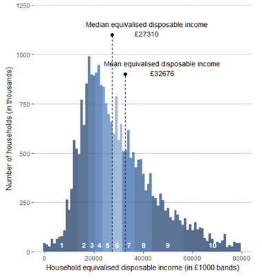
This bulletin looks at two main measures of average household income: the mean and the median. Figure 1 shows the distribution of equivalised disposable income for FYE 2017, clearly indicating the skewness of the distribution; the mean income level (£32,700) is greater than the median (£27,300). The greatest number of households (modal class) falls into the £17,000 to £18,000 bracket, which is in the third decile of the distribution.
Figure 1: Distribution of UK household disposable income, financial year ending 2017
UK
Source: Office for National Statistics
Download this image Figure 1: Distribution of UK household disposable income, financial year ending 2017
.png (46.9 kB) .xls (30.2 kB)
The mean simply divides the total income of households by the number of households. A limitation of using the mean is that it can be influenced by just a few households with very high incomes and therefore does not necessarily reflect the standard of living of the “typical” household. However, when breaking down changes in income and direct taxes by income decile or types of households, the mean allows for these changes to be analysed in an additive way.
Many researchers argue that growth in median household incomes provides a better measure of how people’s well-being has changed over time. The median household income is the income of what would be the middle household, if all households in the UK were sorted in a list from poorest to richest. As it represents the middle of the income distribution, the median household income provides a good indication of the standard of living of the “typical” household in terms of income.
What is disposable income?
Disposable income is arguably the most widely used household income measure. Disposable income is the amount of money that households have available for spending and saving after direct taxes (such as Income Tax, National Insurance and Council Tax) have been accounted for. It includes earnings from employment, private pensions and investments as well as cash benefits provided by the state.
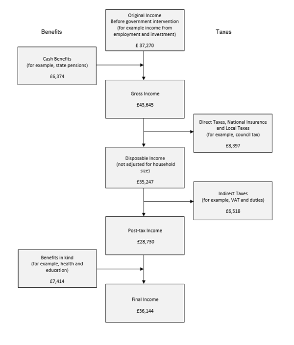
Stages in the redistribution of income
The five stages (Figure 2) are:
Household members begin with income from employment, private pensions, investments and other non-government sources. This is referred to as “original income”.
Households then receive income from cash benefits. The sum of cash benefits and original income is referred to as “gross income”.
Households then pay direct taxes. Direct taxes, when subtracted from gross income is referred to as “disposable income”.
Indirect taxes are then paid via expenditure. Disposable income minus indirect taxes is referred to as “post-tax income”.
Households finally receive a benefit from services (benefits in kind). Benefits in kind plus post-tax income is referred to as “final income”.
Note that at no stage are deductions made for housing costs.
Figure 2: Stages in the redistribution of income
Source: Office for National Statistics
Download this image Figure 2: Stages in the redistribution of income
.png (53.1 kB)
What does it mean for a benefit or tax to be progressive?
A tax is progressive when high-income groups face a higher average tax rate than low-income groups. If those with higher incomes pay a higher amount but still face a lower average tax rate, then the tax is considered regressive; similarly, cash benefits are progressive where they account for a larger share of low-income groups’ income.
Comparisons over time
This bulletin looks at how main estimates of household incomes and inequality have changed over time. To make robust comparisons historic data have been adjusted for the effects of inflation and are equivalised to take account of changes in household composition. More information on the details of these adjustments can be found in the Quality and methodology section of this bulletin.
Estimates in this release are not based on a longitudinal data source so the composition of households differs between periods of time. When growth rates are quoted, they compare the average for a group of households in one period to the average for a different set of households in the next period.
Statistical significance
Statistical significance measures how likely it is that we would see results by chance under the “null hypothesis”, which is the default assumption. In the case of ETB, a common null hypothesis is that no change has occurred in a given statistic between two years (for example, a change in the Gini coeffici from last year to the current year). The phrase "statistically significant at the 5% level" indicates that, if chance alone was operating, a result like this would occur less than 5 times in 100, or less than 5% of the time.
Data periods
Data from the Living Costs and Food Survey used in this analysis are based upon financial years: April to March.
Back to table of contents3. How much do taxes and benefits affect the distribution of income?
Figure 3: Original, gross and disposable income by quintile groups, all households, financial year ending 2017
UK
Source: Office for National Statistics
Download this image Figure 3: Original, gross and disposable income by quintile groups, all households, financial year ending 2017
.PNG (24.1 kB) .xlsx (14.2 kB)
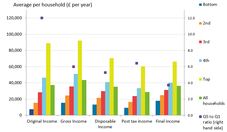
Overall, taxes and benefits lead to income being shared more equally between households. In the financial year ending (FYE) 2017, before direct taxes and cash benefits, the richest fifth (those in the top income quintile group) had an average original income 12 times larger than the poorest fifth – £88,800 per year compared with £7,400 (Figure 3). (Original income includes earnings, private pensions1, and investments.) This factor is unchanged since FYE 2016, indicating that inequality of original income has stayed the same, according to this measure.
Taking account of cash benefits that households received and direct taxes paid resulted in an increase in the income for the poorest fifth of households by £6,000 – to £13,400 - and a decrease in the income of the richest fifth of £18,000 – to £70,700. Consequently, the ratio of income of the richest fifth to the poorest fifth falls from twelve to one, to five to one. The inclusion of indirect taxes (for example, alcohol duties, Value Added Tax (VAT) and so on) and benefits-in-kind (for example, education, National Health Service) further reduces this ratio to less than four to one.
Figure 4: Summary of the effects of taxes and benefits by quintile groups, on all households, financial year ending 2017
UK
Source: Office for National Statistics
Download this chart Figure 4: Summary of the effects of taxes and benefits by quintile groups, on all households, financial year ending 2017
Image .csv .xlsThe diminishing of the ratio of the income between the richest fifth to poorest fifth of households from twelve to one, to less than four to one is explained by comparing the composition of taxes and benefits of these two groups of households. Figure 4 shows that the poorest fifth of households received relatively larger amounts of both cash benefits and benefits-in-kind in FYE 2017. Richer households, on the other hand, paid higher amounts in taxes – both direct and indirect.
Back to table of contents4. Indirect taxes increase inequality of income
Household disposable income and inequality in the UK: financial year ending (FYE) 2017 presented detailed analysis on the value and composition of direct taxes and cash benefits paid and received by different groups of households in the income distribution. It showed that poorer households were more likely to be in receipt of cash benefits, in particular those relating to employment, and tax credits.
Further, the second-poorest fifth of households received, on average, more cash benefits than the poorest fifth of households. This is due largely to the State Pension, which in this analysis is classified as a cash benefit, making up the largest proportion of the total cash benefits received by households and there are, on average, more retired people in households in the second quintile group than the bottom group.
The richest fifth of households paid on average £21,400 in direct taxes in FYE 2017, the majority of which (almost 70%) was Income Tax. This corresponds to 23.2% of their gross income, broadly unchanged from other recent years. The average direct tax bill for the poorest fifth was £1,900, of which the largest component, over half, was Council Tax or Northern Ireland rates. This was equivalent to 12.7% of gross household income for this group, slightly higher than in FYE 2016 (11%).
This release provides more detailed analysis on indirect taxes (such as Value Added Tax (VAT) and duties on alcohol and fuel) and benefits-in-kind (for example, NHS and state-provided education). Indirect taxation is determined by households’ expenditure rather than their income. The richest fifth of households paid nearly three times as much in indirect taxes as the poorest fifth (£10,300 and £4,000 per year, respectively). This reflects greater expenditure on goods and services subject to these taxes by higher-income households.
Figure 5: Indirect taxes and benefits-in-kind as a proportion of disposable income by quintile groups, ALL households, financial year ending 2017
UK
Source: Office for National Statistics
Download this chart Figure 5: Indirect taxes and benefits-in-kind as a proportion of disposable income by quintile groups, ALL households, financial year ending 2017
Image .csv .xlsHowever, although richer households pay more in indirect taxes than poorer ones in total, they pay less as a proportion of their income. The poorest fifth of households paid almost 30% of their disposable income in indirect tax – with VAT (12.8%) being the biggest component – compared with 14.6% of disposable income for the richest fifth of households. This means that indirect taxes increase inequality of income.
Across all households, there was a 6.4% increase in the average value of indirect taxes paid between FYE 2016 and FYE 2017. More than half of this growth (3.5 percentage points) was accounted for by an increase in the amount of VAT that households pay. Given that there had been no policy changes in VAT rates, or VATable goods, this growth was accounted for by stronger growth in expenditure of VATable goods. This is explored in greater detail further on in the bulletin.
The only other significant contributor to growth in indirect taxes was Employers’ National Insurance Contributions (1.4 percentage points). This is likely to be an employment effect – there has been an associated increase in the amount of Income Tax paid, and wages and salaries received between FYE 2016 and FYE 2017 after accounting for the effects of inflation.
Benefits-in-kind increase the equality of income. Benefits-in-kind are goods and services provided by the government to households that are either free at the time of use or at subsidised prices, such as education and health services. These goods and services can be assigned a monetary value based on the cost to the government, which is then allocated as a benefit to individual households.
The poorest fifth of households received benefits in-kind equivalent to 62.8% of disposable income, with the National Health Service (35.4%) and education (25.4%) being the two largest contributors. The richest fifth of households, on the other hand, received benefits-in-kind equivalent to 8.4% of disposable income, again NHS (6.0%) and education (2.0%) the largest contributors.
The poorest fifth of households receive more education-related benefit-in-kind in total and, therefore, as a proportion of their income. This is largely because households towards the bottom of the income distribution have, on average, a larger number of children in state education.
While the poorest fifth of households receive a higher proportion of their income in NHS-related benefit in kind, they received a similar amount in total to the richest fifth in FYE 2017 (£4,700 and £4,200 respectively). Our current methodology for allocating NHS spending to individuals is based on age and sex. Given that there are no substantial differences in the composition of households, in terms of age and sex, across the income distribution, NHS spending is allocated fairly evenly. We plan to update our methodology for allocating NHS spending, which will take better account of the relationship between deprivation and increased use of the health services (Asaria, Doran, & Cookson, 2016).
Overall, the impact of benefits-in-kind more than offset the increase in income inequality caused by indirect taxes. As mentioned earlier, the ratio of disposable income of richest fifth to the poorest fifth in FYE 2017 is five to one. This ratio increases to six to one on a post-tax income basis (disposable income minus indirect taxes), but then falls to less than four to one on a final income basis (post-tax income plus benefits in kind).
Back to table of contents5. Cash benefits have the largest effect on reducing income inequality
There are various ways in which inequality of household income can be assessed – including the ratio of average income of the top and bottom fifth of households presented earlier. Perhaps the most widely used measure internationally is the Gini coefficient. Gini coefficients can vary between zero and 100 and the lower the value, the more equally household income is distributed. One of the advantages of the Gini coefficient is that it considers the whole distribution, rather than, for instance, just the tails.
Figure 6: Impact of cash benefits and taxes on Gini coefficient, financial year ending 2017
UK

Source: Office for National Statistics
Download this image Figure 6: Impact of cash benefits and taxes on Gini coefficient, financial year ending 2017
.png (13.4 kB) .xls (32.8 kB)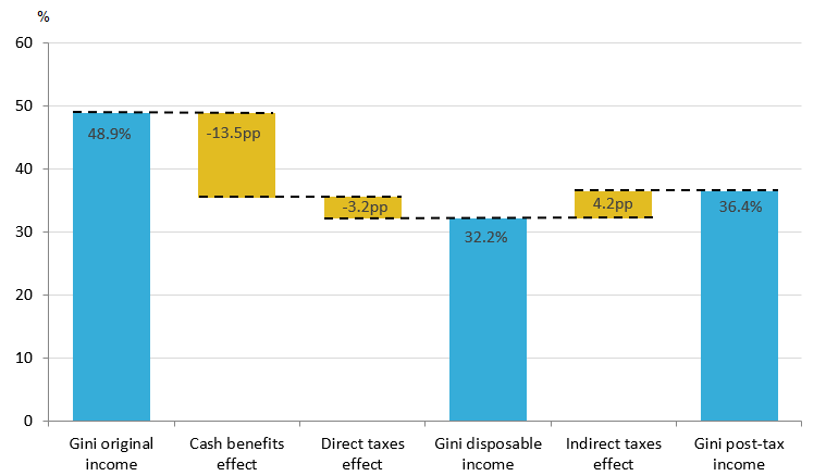
The extent to which cash benefits, direct taxes and indirect taxes work together to affect income inequality can be seen by comparing the Gini coefficients of original, gross, disposable and post-tax incomes.
Cash benefits had the largest effect on reducing income inequality, in the financial year ending (FYE) 2017, reducing the Gini coefficient by 13.5 percentage points from 48.9% for original income to 35.4% for gross income (Figure 6). Direct taxes acted to further reduce it, by 3.4 percentage points to 32.2%. As described earlier, indirect taxes act to increase income inequality – the Gini coefficient of post-tax income was 4.2 percentage points higher than the Gini coefficient of gross income (36.4% and 32.2% respectively). This means that overall, taxes had a negligible effect on income inequality.
Table 1: Changes in Gini coefficients
| Gini coefficients (%) | ||||
|---|---|---|---|---|
| Original Income | Gross Income | Disposable Income | Post-tax Income | |
| Financial year ending 2016 | 49.3 | 35.0 | 31.6 | 35.4 |
| Financial year ending 2017 | 48.9 | 35.4 | 32.2 | 36.4 |
| Change | -0.4 | 0.4 | 0.6 | 1.0 |
| Source: Office for National Statistics | ||||
Download this table Table 1: Changes in Gini coefficients
.xls (27.1 kB)While cash benefits had the largest impact on reducing income inequality in FYE 2017, this effect may have diminished between FYE 2016 and 2017. As highlighted in Table 1, the estimated Gini coefficient of disposable income grew at a faster rate than the estimated Gini coefficient of gross income (0.6 percentage points and 0.4 percentage points respectively). In addition, the Gini coefficient of post-tax income is estimated to be growing at a faster rate than disposable income, implying that indirect taxes may have become more regressive between FYE 2015 and FYE 2016.
Figure 7: Change in the proportion of the total of each income component by quintile, financial year ending 2016 to financial year ending 2017
UK
Source: Office for National Statistics
Download this chart Figure 7: Change in the proportion of the total of each income component by quintile, financial year ending 2016 to financial year ending 2017
Image .csv .xlsWhile changes in the estimated Gini coefficients compared with last year, are not statistically significant, it is interesting nonetheless to explore the contributing factors behind their divergence. To better examine the potential diminished effect of cash benefits at reducing income inequality between FYE 2016 and FYE 2017, Figure 7 presents the change in the share of the total of each income component that each quintile received over this time period. While the poorest fifth of households increased their share of total cash benefits (from 24% to 24.9%), the second income quintile saw their share reduced (from 30.4% to 28.5%). Overall this meant that the poorest 50% of households reduced their share by 1.5 percentage points from 66.3% to 64.7% (Figure 8).
The poorest half of households also increased their share of total indirect taxes paid – by 1.0 percentage point, from 34.5% to 35.6% – helping to explain the potential increased regressivity of indirect taxes between FYE 2016 and FYE 2017.
Figure 8: Change in composition of cash benefits received by poorest 50% of households between financial year ending 2016 to financial year ending 2017
Financial year ending 2017 prices, UK

Source: Office for National Statistics
Download this image Figure 8: Change in composition of cash benefits received by poorest 50% of households between financial year ending 2016 to financial year ending 2017
.PNG (11.3 kB) .xlsx (16.4 kB)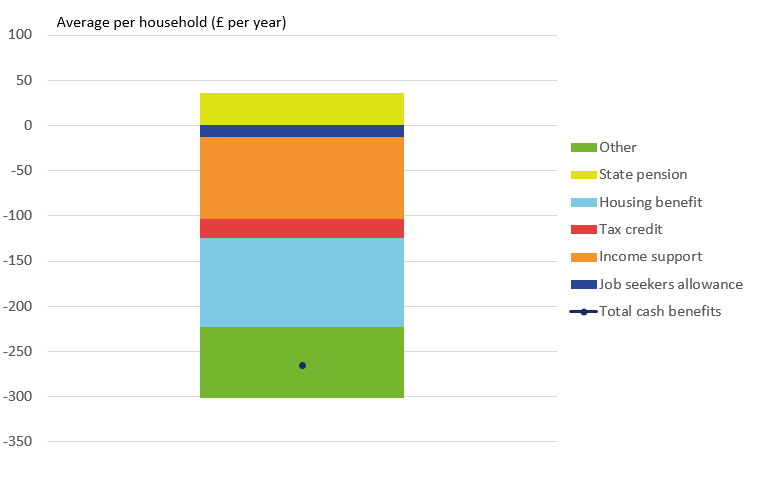
Between FYE 2016 and FYE 2017, the average amount of cash benefits that the poorest half of households received is estimated to have fallen by £270, after accounting for the effects of inflation (Figure 8).
Figure 9: Change in composition of indirect taxes paid by poorest 50% of households between financial year ending 2016 and financial year ending 2017, in financial year ending 2017 prices
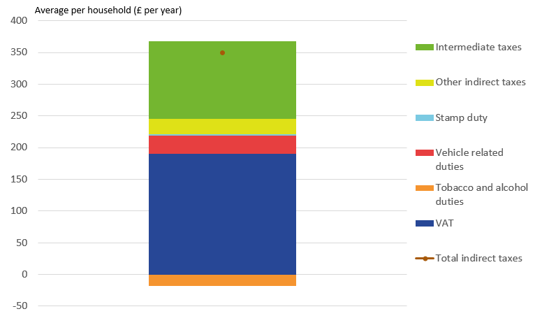
Source: Office for National Statistics
Download this image Figure 9: Change in composition of indirect taxes paid by poorest 50% of households between financial year ending 2016 and financial year ending 2017, in financial year ending 2017 prices
.PNG (12.3 kB) .xlsx (15.6 kB)
The average value of indirect taxes paid by the poorest 50% of households was estimated to have increased by £350 between FYE 2016 and FYE 2017 after accounting for the effects of inflation. This was driven primarily by growth in the average amount of Value Added Tax (VAT) (£190) and intermediate taxes (£120) that households paid.
Figure 10: Contributions to growth in amount of value added tax paid by type of expenditure, income quintile, financial year ending 2016 to financial year ending 2017
UK
Source: Office for National Statistics
Download this chart Figure 10: Contributions to growth in amount of value added tax paid by type of expenditure, income quintile, financial year ending 2016 to financial year ending 2017
Image .csv .xlsFigure 10 examines the growth in VAT paid for poorer households, as well as the wider income distribution, in more detail. It shows that overall, most households paid more VAT in FYE 2017 compared with FYE 2016 after accounting for the effects of inflation. This reflects the analysis provided within this year’s Family spending reporting that average weekly household spending return to its pre-economic downturn levels for the first time.
The amount of VAT paid by the poorest fifth and second-poorest fifth of households increased by 14.1% and 12.8% respectively. For the poorest fifth of households, this growth was driven by recreation, hotels and restaurants, and transport expenditure (5.6 percentage points and 3.0 percentage points respectively).
Figure 11: Gini coefficients for original, disposable income, and final income, 1977 to financial year ending 2017
UK
Source: Office for National Statistics
Notes:
- Equivalised using the modified-OECD scale.
- An improved process for calculating the Gini coefficient has been implemented which has resulted in a change to the levels of rounding applied. Although not significant, there are minor differences to previously published Gini estimates.
Download this chart Figure 11: Gini coefficients for original, disposable income, and final income, 1977 to financial year ending 2017
Image .csv .xlsThe Gini coefficient on disposable income increased by 0.6 percentage points between FYE 2016 and FYE 2017, from 31.6% to 32.2%. The Gini coefficient on post-tax income increased by 1.0% over the same period, from 35.4% to 36.4% (Figure 11).
The change in Gini coefficient on disposable income between FYE 2016 and FYE 2017 is not statistically significant, meaning that there is little confidence that income inequality has changed between these years. In fact, the Gini coefficient on disposable income has been relatively stable over the past 10 years, falling by an average of 0.3 percentage points per year between FYE 2007 and FYE 20171. This is a continuation of the trend seen since 1990 (calendar year) where the Gini coefficient on disposable income fell by an average of 0.2 percentage points, from 36.8% to 32.2%. This contrasts significantly with the period spanning late 1977 up to 1990, where the Gini coefficient increased by 0.9 percentage points per year, from 26.6% to 36.8%.
Figure 12: S80/S20 ratio for disposable income, 1977 to financial year ending 2017
UK
Source: Office for National Statistics
Download this chart Figure 12: S80/S20 ratio for disposable income, 1977 to financial year ending 2017
Image .csv .xlsAnother measure of income inequality is the S80/S20 ratio. This measure is equal to the average disposable income for the richest 20% of households divided by the average disposable income for the poorest 20% of households – a higher S80/S20 ratio means that households are more unequal. While some year-on-year movements reflect survey volatility, it appears that the S80/S20 ratio increased from 1977 to 1990, where it reached a peak of 6.4. The rate of increase was highest during the mid-1980s. There appears to have been a gradual decline in S80/S20 inequality from 1991 to 2017 (Figure 12).
Figure 13: Cumulative contributions to growth in equivalised household disposable income from 1977 to financial year ending 1991 and financial year ending 1992 to financial year ending 2017, top and bottom income quintiles
Financial year ending 2017 prices, UK
Source: Office for National Statistics
Download this chart Figure 13: Cumulative contributions to growth in equivalised household disposable income from 1977 to financial year ending 1991 and financial year ending 1992 to financial year ending 2017, top and bottom income quintiles
Image .csv .xlsFigure 13 shows that for the richest fifth of households, incomes grew at a faster rate compared with the poorest fifth between 1978 and FYE 1991. This growth was driven mainly by increases in original income. In absolute terms, higher-income households paid more direct taxes in FYE 1991 than they did in 1978 and received about the same amount in cash benefits.
For the poorest fifth of households, incomes grew more slowly from 1978 to FYE 1991. Growth was driven mainly by increases in the amount of cash benefits received. In absolute terms, poorer households had lower original incomes and paid more in direct taxes in FYE 1991 than in 1978.
From FYE 1992 to FYE 2017, disposable income growth rates were more comparable – growth among the poorest fifth of households slightly exceeded that of the richest fifth. For both groups, disposable income growth was driven primarily by increases in wages, and pension and annuity amounts. In absolute terms, high-income and low-income households each received more in cash benefits and paid more direct tax in FYE 2016 than in FYE 1991.
More detailed analysis of the impact of taxes and benefits on inequality over time using a range of measures can be found in the article The effects of taxes and benefits on income inequality, 1977 to financial year ending 2015.
Notes for: Cash benefits have the largest effect on reducing income inequality
- DWP’s Households below average income (HBAI) statistics have an alternative Gini series, which shows a stable picture in recent years. HBAI includes an adjustment for high-income individuals based on tax records, whose incomes tend to be under-reported on voluntary surveys. Changes in the incomes of the very richest may have contributed to the differences in trends between these two sources.
6. Households where the head is aged between 25 and 64 years paid more in taxes than they received in cash and in-kind benefits
Figure 14: The effects of taxes and benefits by age of the household reference person, financial year ending 2017
UK
Source: Office for National Statistics
Notes:
- The household reference person is the householder who:
- owns the household accommodation, or
- is legally responsible for the rent of the accommodation, or
- has the household accommodation as an emolument or perquisite, or
- has the household accommodation by virtue of some relationship to the owner who is not a member of the household.
If there are joint householders the household reference person will be the one with the higher income. If the income is the same, then the eldest householder is taken.
Download this chart Figure 14: The effects of taxes and benefits by age of the household reference person, financial year ending 2017
Image .csv .xlsThe effects of taxes and benefits were felt differently by households in different age groups (Figure 14). On average, in the financial year ending (FYE) 2017, households with a household head aged between 25 and 64 years paid more in taxes (direct and indirect) than they received in benefits (including in-kind benefits), whilst the reverse was true for those aged 65 years and over. Households where the head was aged 50 to 54 years paid the most in taxes (£20,300). Households where the main earner was in their early 40s, were the third-highest in terms of taxes paid (£19,200 on average). However, they also received the highest average amount in benefits of those below State Pension age (£16,000), due mainly to the benefit in-kind received from state-provided education (£7,000).
For households where the main earner is aged 65 years and over, the State Pension and Pension Credit was the largest component of the benefits received, followed by the benefit derived from the National Health Service, which becomes increasingly important as age increases. Those households with heads under the age of 25 years were the other age group who, on average, received more in benefits than they paid in taxes.
Figure 15: Change in average amount per household in taxes paid or benefits received, and net position, by age of household reference person, financial year ending 2007 to financial year ending 2017
Source: Office for National Statistics
Download this chart Figure 15: Change in average amount per household in taxes paid or benefits received, and net position, by age of household reference person, financial year ending 2007 to financial year ending 2017
Image .csv .xlsFigure 15 compares changes in the average value of benefit received or tax paid by age of head of the household between FYE 2007 and FYE 2017, after adjusting for the effects of inflation. Three main observations emerge.
First, households where the head is aged between 30 and 49 years increased their net position over the 10-year period. This was driven mainly by a decrease in the average amount of total direct and indirect taxes paid, and an increase in the benefits-in-kind received from state-provided education.
Second, households where the main earner is aged between 60 and 69 years have seen a worsening of their net position over the 10 years between FYE 2007 and FYE 2017. For households where the head of household is aged 60 to 64 years, this worsening was due to a fall in the amount of State Pension received. This likely reflects in part the increasing State Pension age for women over this period.
Households where the head of the household is aged between 65 to 69 years have seen a large increase in the average amount of taxes and indirect taxes paid. This was driven partly by increases in the amount of State Pension received and a rise in original income for over 65s since last year, since these are both liable to Income Tax. However, most of the change was attributable to increases in the amount paid towards indirect taxation. Increased activity levels in the employment market do not appear to be the cause, as the proportion of over 65s in employment, actively looking for work, or taking part in work-based training schemes has fallen slightly from FYE 2016.
Finally, households where the main earner is aged 65 years and over have seen an increase in the average amount of State Pension received. This was likely a combination of the introduction of State Pension Credit, coupled with the impact of the “triple lock”1, which has ensured real terms growth in recent years.
Notes for: Households where the main earner is aged between 25 and 64 years paid more in taxes than they received in cash and in-kind benefits
- The triple lock was introduced in 2010 to guarantee to increase the State Pension every year by the higher of inflation, average earnings or a minimum of 2.5%.
7. Policy context: changes to taxes in FYE 2017
This section provides information for some of the main changes to taxes (direct and indirect) in the financial year ending (FYE) 2017.
National Insurance
From 6 April 2016, individuals are no longer able to contract out of the additional State Pension (also known as second State Pension or SERPS). This allowed those paying into a pension scheme to pay a reduced rate of National Insurance (NI); for employees this was a 1.4% reduction (on a proportion of earnings). This also means that employers no longer receive a 3.4% rebate for any employees in contracted-out pension schemes. In FYE 2017, employees who previously qualified for a reduced rate would have seen an increase in their NI.
Stamp Duty
From April 2016, a 3% surcharge on existing Stamp Duty Land Tax rates is applied to those buying a second home and those investing in buy-to-let properties.
Air Passenger Duty
From April 2016, Air Passenger Duty rates for flights originating from UK airports changed. Band B, which covers destinations over 2,000 miles from London, had an increase of £2 on the reduced rate, which covers travel in the lowest class available on an aircraft, and £4 on the standard rate, which relates to travel in any other class of travel.
Insurance Premium Tax
Insurance Premium Tax (IPT) increased by 0.5 percentage points to 10% from 1 October 2016.
Back to table of contents8. Economic context
For more information about how these statistics fit the wider UK economic perspective see the Economic context section of the latest edition of Household disposable income and inequality in the UK.
Back to table of contents9. Quality and methodology
The effects of taxes and benefits on household income Quality and Methodology Information report contains important information on:
the strengths and limitations of the data and how it compares with related data
uses and users of the data
how the output was created
the quality of the output including the accuracy of the data
Analysis in this bulletin is based on our long-running Effects of taxes and benefits on household income (ETB) series. The ETB series has been produced each year since the early 1960s. Historical tables, including data from 1977 onwards are also published today, along with the Consumer Prices Index including owner-occupiers’ housing costs (CPIH), which can be applied to adjust for the effects of inflation. Differences in the methods and concepts used mean that it is not possible to produce consistent tables for the years prior to 1977 and only relatively limited comparisons are possible for these early years. All comparisons with previous years are also affected by sampling error.
Back to table of contents10. Glossary
Equivalisation
Income quintile groups are based on a ranking of households by equivalised disposable income. Equivalisation is the process of accounting for the fact that households with many members are likely to need a higher income to achieve the same standard of living as households with fewer members. Equivalisation takes into account the number of people living in the household and their ages, acknowledging that while a household with two people in it will need more money to sustain the same living standards as one with a single person, the two-person household is unlikely to need double the income.
This analysis uses the modified-Organisation for Economic Co-operation and Development (OECD) equivalisation scale (PDF, 165KB).
Gini coefficients
The most widely used summary measure of inequality in the distribution of household income is the Gini coefficient. The lower the value of the Gini coefficient, the more equally household income is distributed. A Gini coefficient of zero would indicate perfect equality where every member of the population has exactly the same income, while a Gini coefficient of 100 would indicate that one person has all the income.
Income quintiles
Households are grouped into quintiles (or fifths) based on their equivalised disposable income. The richest quintile is the 20% of households with the highest equivalised disposable income. Similarly, the poorest quintile is the 20% of households with the lowest equivalised disposable income. Given households vary in size, quintiles contain differing numbers of individuals.
Household income
This analysis uses several different measures of household income. Original income (before taxes and benefits) includes income from wages and salaries, self-employment, private pensions and investments. Gross income includes all original income plus cash benefits provided by the state. Disposable income is that which is available for consumption and is equal to gross income less direct taxes.
Retired persons and households
A retired person is defined as anyone who describes themselves (in the Living Costs and Food Survey) as “retired” or anyone over minimum National Insurance pension age describing themselves as “unoccupied” or “sick or injured but not intending to seek work”. A retired household is defined as one where the combined income of retired members amounts to at least half the total gross income of the household.
Back to table of contents11. Users and uses of these statistics
The effects of taxes and benefits on household income (ETB) statistics are of particular interest to HM Treasury (HMT), HM Revenue and Customs (HMRC) and the Department for Work and Pensions (DWP) in determining policies on taxation and benefits, and in preparing budget and pre-budget reports. Analyses by HMT based on this series, as well as the underlying Living Costs and Food (LCF) dataset, are published alongside the budget and autumn statement. A dataset, based on that used to produce these statistics, is used by HMT in conjunction with the Family Resources Survey (FRS) in their Intra-Governmental Tax and Benefit Microsimulation Model (IGOTM). This is used to model possible tax and benefit changes before policy changes are decided and announced.
In addition to policy uses in government, the ETB statistics are frequently used and referenced in research work by academia, think-tanks and articles in the media. These pieces often examine the effect of government policy, or are used to advance public understanding of tax and benefit matters. The data used to produce this release are made available to other researchers via the UK Data Service.
These statistics play an important role in providing an insight to the public on how material living standards and the distributional effect of government policy on taxes and benefits have changed over time for different groups of households.
Back to table of contents