Table of contents
- Overview
- Introduction to death registration and occurrences data
- Exploring the relationship between death occurrence and registration
- Predicting death occurrences from up to three weeks registration data
- Caveats of the approach
- Appendix 1: Relationship between death registrations and death occurrences
- Appendix 2: Modelling registration delay
- Appendix 3: Measuring performance against 2019 data
- Related links
1. Overview
Registration delays
Deaths are not generally registered on the actual date of death, so there is a delay between occurrence and registration. We regularly publish analysis of these registration delays. These registration delays make it difficult for us to report timely and complete statistics on death occurrences as the total number of deaths that occurred in a given week can only be known some time later. For this reason, we have historically published weekly counts of death registrations rather than death occurrences.
In exceptional situations there can be excess deaths brought about by environmental factors such as the weather or disease, as seen in the coronavirus (COVID-19) pandemic. A method to estimate the total number of deaths occurring based on the limited registration data available is therefore of value.
We publish this method with the intention of using it in the future to help inform analyses needing time-sensitive monitoring of numbers of deaths. The most appropriate way of publishing such estimates is still being considered. This method is experimental and no estimates relating to deaths in 2020 are included in the paper.
Weekly data on deaths
To have clear information on trends in deaths in the short-term, it is useful to estimate the number of deaths in the most recent weeks.
In our weekly deaths publications we report the number of deaths that were registered within a particular week in England and Wales. We report each Tuesday on the deaths registered in the week ending on the Friday 11 days before.
From week 13 2020 (week ending 27 March, published 7 April 2020), because of the increased need for data on deaths during the coronavirus (COVID-19) pandemic, we started reporting the number of deaths involving COVID-19 by date of occurrence as well as date of registration, including deaths occurring in the reference week that are registered as close to the publication date as possible (usually 10 days after the end of the reporting week). However, figures reported by date of occurrence relatively soon after the date of death are incomplete because of the known delays.
Relationship between death occurrences and registrations
In this article, the relationship between weekly total death occurrences and registrations of those deaths occurring in the same week and those immediately following is investigated. The method outlined uses patterns of registration delay from previous years to estimate the number of deaths likely to have occurred in a time period but not yet been registered and produces an estimated total number of deaths that occurred within a specific week with confidence intervals. The further in time from the week of interest, the more complete the data and the more accurate the estimated total number.
This method also takes account of weeks that include bank holidays, when there is greater delay because of closed services.
Based on data covering years 2015 to 2018, it is found that means of around:
- 46% of deaths are registered in the same week as occurrence
- 85% are registered by the end of the subsequent week
- 91% are registered by the end of the subsequent second week
Simply speaking the reciprocal of these values can be applied to current registration data to estimate the true numbers of occurrences. Here the role of seasonal factors such as holiday periods on the variation of these registration rates is explored.
Results and recommendations
It is found that bank holidays have a strong effect on reducing the rate of registration in the same week and immediately adjacent weeks. It is also found that there is a seasonal effect on registration rates that correlates with the seasonal increase in death occurrences. This compromises the approach to the extent that increased deaths could result in a reduction in the rate of registration and an under-estimate of total deaths. In addition, the method assumes that current registration patterns follow historical norms, an assumption that may not hold in all circumstances.
Relatively simple models of registration delay can be used to estimate the total number of occurrences based on early registration data. Application of these models including seasonal and bank holiday effects based on 2015 to 2018 data to predict total death data in 2019 showed strong performance and utility. A predictive accuracy of within 3% is observed when estimating total deaths from registrations occurring in the same week, improving to 0.7% when estimating total deaths from cumulative registrations by end of the subsequent week (based on mean absolute error). There is evidence that excess deaths resulting from time specific events such as a heatwave can be predicted from cumulative registrations by end of the subsequent week.
Back to table of contents2. Introduction to death registration and occurrences data
Registration of deaths is not instantaneous. To register a death in England and Wales either a medical certificate of death or permission from a coroner is required. According to the Births and Deaths Registration Act 1953, unless the death is referred to a coroner, it should be registered within five calendar days. There is no time restriction placed on coroners to provide permission to register a death once it has been referred, and because of the time that can be needed to hold an inquest, registration may be weeks, months or even years after the death has occurred. The time between death occurring and being registered is referred to as registration delay. In 2018, the median registration delay in England and Wales was five days.
Once a death is registered at the local registration office, the data are sent overnight to the Office for National Statistics (ONS) and are available for coding within two working days and usually for analysis on the third working day. The ONS publishes weekly provisional death registrations every Tuesday. These data are for the week ending on the Friday 11 days earlier and are extracted from ONS systems on the following Thursday.
Weekly counts of deaths are published using date of registration of the death because all registrations for the week are usually captured; the data do not usually need to be revised and so can be released in a timely fashion. However, generally only about 46% of registered deaths occurred in the same registration week, with a further 39% occurring in the week before (based on mean values for 2018). Most of the remaining registrations are for deaths that have been referred to a coroner and occurred more than four weeks earlier. So weekly registered deaths cover a large period of when the death occurred.
This article investigates the practicality of publishing weekly death occurrences, bearing in mind that the ONS does not know about a death until it is registered. As a proportion of all occurrences, the number of deaths registered over time becomes ever closer to the true value. The question investigated is how many weeks of registration data are required following an occurrence week for us to precisely estimate the total number of deaths that occurred in that week? This requires understanding of the variation of registration rates by week delay so that the amount of unexplained variation in rates is small and concomitantly our confidence intervals are narrow. This question will be particularly useful in estimating excess deaths that occur because of time-specific events.
The current reporting of weekly death registrations has limited use for time-sensitive surveillance but can be produced at speed. We show that it is possible to estimate weekly death occurrences with high accuracy and precision (narrow confidence intervals) using the limited registration data that are available by the end of the week following the week of occurrence.
Looking for information on the coronavirus?
3. Exploring the relationship between death occurrence and registration
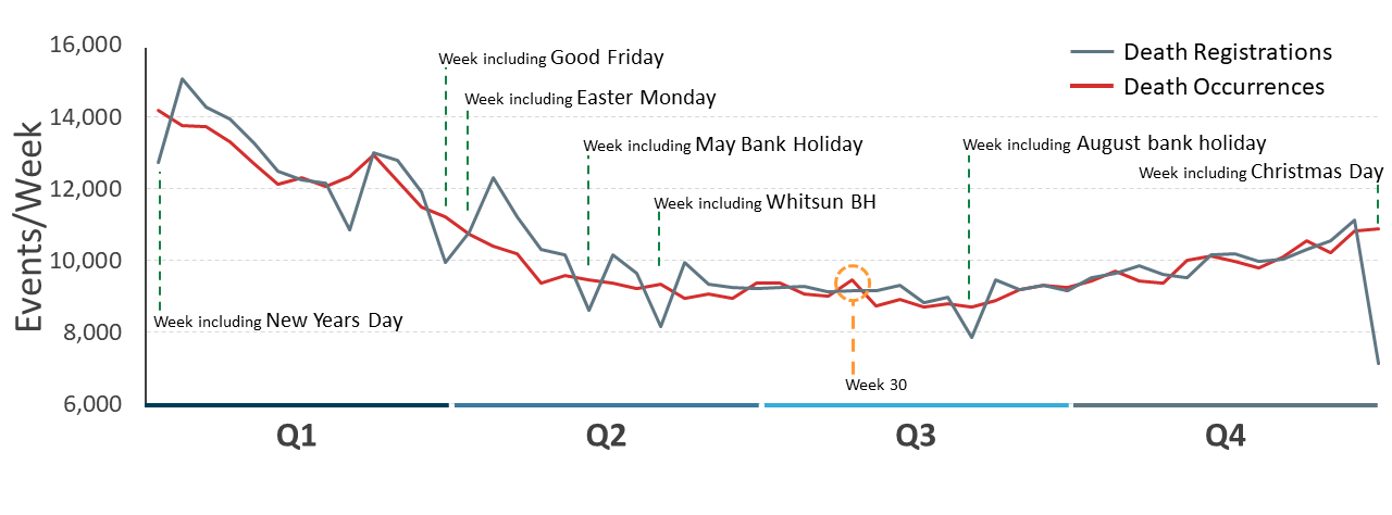
The weekly death registration data that the Office for National Statistics (ONS) publishes define a week as running from Saturday to Friday. The weekly account of death occurrences and registrations for 2018 in England and Wales is shown in Figure 1.
The number of death registrations during a week containing bank holidays is typically reduced by around 10% and there is a bounce of increased registrations most obviously in the subsequent week.
Figure 1: Death registrations are affected by bank holidays
Number of deaths occurring and registered by week in 2018, England and Wales
Source: Office for National Statistics
Notes:
- Week 1 begins Saturday 30 December 2017.
- The hottest day of 2018 was recorded in week 30.
Download this image Figure 1: Death registrations are affected by bank holidays
.png (61.5 kB)
The daily account of death occurrences and registrations for 2018 in England and Wales using the same data is shown in Figure 2. Daily registrations show a weekly pattern, with a peak on a Tuesday and few or no registrations at the weekend or on bank holidays (Figure 2; note that the weekly peak of registrations is pushed to a Wednesday following a bank holiday Monday). So death registrations are most obviously affected by available working days, though it is also clear that there are more death registrations in winter than in summer months.
In contrast, there is little evidence that being a working day, or a specific weekday, affects the number of deaths that occur. However, as for registrations, the number of deaths occurring is higher in winter than in the summer months.
Figure 2: Number of death registrations varies by day of the week.
Number of deaths occurring and registered by day in 2018, England and Wales.

Source: Office for National Statistics
Notes:
- Aligned to Figure 1; week 1 begins Saturday 30 December 2017.
- The hottest day of 2018 was recorded on 27 July.
- Vertical bars represent bank holidays.
Download this image Figure 2: Number of death registrations varies by day of the week.
.png (75.7 kB)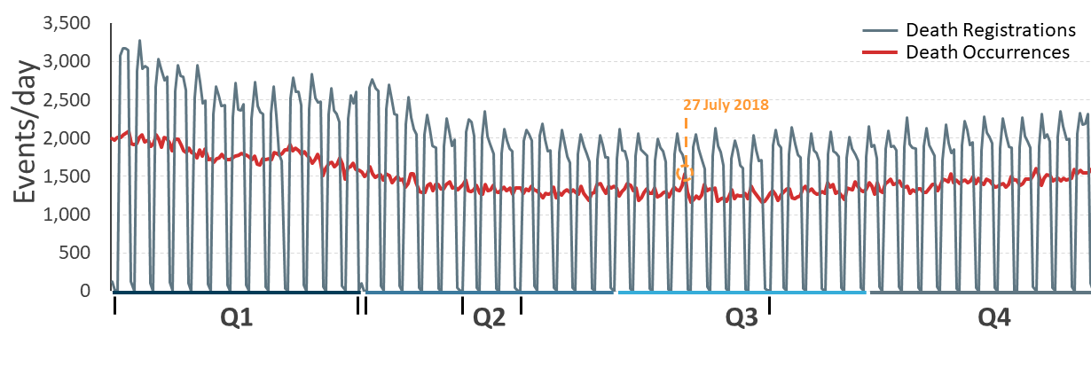
The hottest day of 2018 was Friday 27 July, with 35.6 degrees Celsius recorded in Felsham, Suffolk. This event does not produce an observable effect upon daily or weekly death registrations, but it does coincide with a peak in both the daily and weekly number of death occurrences (day peak occurred on 27 July 2018 (Figure 2, highlighted), weekly peak for week beginning 21 July 2018 (Figure 1, highlighted)). This suggests that to assess the public health impact of rare, time-specific, events it would be more useful to prioritise examination of death occurrence over death registration data.
Measuring variability in the registration delay
The time between the death occurrence and registration is the registration delay. Historic patterns of registration delay can potentially be applied to current registration data to predict the total of death occurrences.
So for a given time X after an occurrence period, historically the mean proportion of those occurrences are registered by that time is px, then the current number of occurrences registered by the same time delay divided by px gives an estimate of the true number of death occurrences in the period of interest. The success of this method depends upon an assumption that the current year will have a similar pattern and variation in registration delay as the historic data. We need to measure the size of this historic variation to ascribe an uncertainty to our estimate. A general caveat to the approach is that registration delay may be correlated with the number of deaths (Appendix 1: Relationship between death registrations and death occurrences).
The problem under investigation is framed as what proportion of deaths occurring within a certain time period are expected to be registered by time X after that period? This analysis is aligned to the publication of weekly provisional death registrations. These weeks begin each Saturday and end on the following Friday. The first week of any given year ends on the first Friday of that year. Deaths can be identified with two weeks: the week in which the death occurred (occurrence period) and the week in which the death was registered (registration delay). The time in weeks between week of occurrence and the week of registration is the delay period in weeks. The analysis covers a delay period of up to five weeks and assumes that all deaths that occurred in any given week in 2015 to 2018 are registered by the end of 2019.
A fuller account of the methodology is given in Appendix 2: Modelling registration delay. In brief, a given week of death occurrences is treated as a set of n trials (deaths) with each trial sharing a probability of πx that each death will be registered at time X. The proportion of deaths (p) that are registered at time X is an estimator of πx, with a variance of p(1-p)/n. As the number of deaths is large (more than 8,000 per week; Figure 1), px is a precise estimator allowing us to ignore the variance of the estimator. The mean and variance of the population of proportions (px) are under investigation here.
This population of proportions is made up of the 52 (or 53) weeks of death occurrences in a year. For the period of analysis, 2015 to 2018, there are 209 weeks. The proportion of deaths that are registered in the same week that they occurred is referred to as p0. The proportion of deaths that are registered by the end of the subsequent week that they occurred in is referred to as p1 and so on to p5, the limit of this study.
As this investigation is a study of a population of proportions, which may not be normally distributed, values undergo the logit transformation (logit px = loge(px/(1-px))). Following this transformation, normality is assumed for analysis and variance calculations. In most cases, values are presented back in the probability scale using the following conversion:
px = 1/(1+exp(-logit(value)))
Overall registration delay between years 2015 and 2018
The mean proportion of deaths registered by weeks delay by year is shown in Table 1 and are calculated through the logit transformation with 95% confidence intervals as shown. For comparison, means calculated without logit transformation are shown in square brackets.
Null models are simply these means (expected values), which can be used to make predictions; the reciprocal of these mean proportions can be used to estimate total occurrences based on registrations by delay week 0 to 5 (Table 1; reciprocal of the lower confidence interval of proportion gives an estimate of the upper confidence of predicted values).
As reported in Impact of registration delays on mortality statistics in England and Wales: 2018, the registration delay appears to lengthen from 2015, suggesting a trend that using historic data to predict current occurrences may systematically under-estimate values (Table 1).
| 2015 | 2016 | 2017 | 2018 | |
|---|---|---|---|---|
| p₀ | 48.6% (40.6% - 56.6%) [48.6%] | 45.7% (37.3% - 54.3%) [45.7%] | 45.5% (37.6% - 53.6%) [45.5%] | 45.5% (36.3% - 55.0%) [45.6%] |
| p₁ | 86.7% (82.9% - 89.8%) [86.6%] | 84.9% (80.5% - 88.3%) [84.7%] | 84.9% (80.3% - 88.6%) [84.8%] | 84.5% (80.2% - 88.0%) [84.4%] |
| p₂ | 91.4% (90.0% - 92.6%) [91.3%] | 90.5% (89.2% - 91.7%) [90.5%] | 90.6% (89.3% - 91.8%) [90.6%] | 90.5% (89.2% - 91.6%) [90.5%] |
| p₃ | 92.3% (91.0% - 93.5%) [92.3%] | 91.8% (90.9% - 92.7%) [91.8%] | 92.0% (91.2% - 92.7%) [92.0%] | 91.9% (90.8% - 92.9%) [91.9%] |
| p₄ | 92.8% (91.6% - 93.9%) [92.8%] | 92.4% (91.4% - 93.2%) [92.4%] | 92.5% (91.7% - 93.3%) [92.5%] | 92.5% (91.4% - 93.5%) [92.5%] |
| p₅ | 93.8% (92.0% - 94.2%) [93.1%] | 92.8% (91.8% - 93.6%) [92.7%] | 92.9% (92.0% - 93.7%) [92.9%] | 92.9% (91.8% - 93.8%) [92.8%] |
Download this table Table 1: The mean proportion of all weekly deaths registered by delay and year, England and Wales, 2015 to 2018
.xls .csvLargest cause of variability in registration delay of deaths is bank holidays
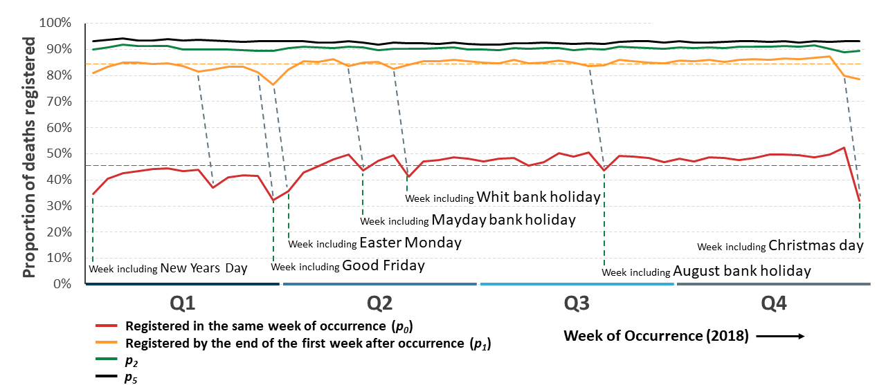
In this section, the rates of registration delay by weeks delay are examined. In Figure 3, the week of occurrence is plotted on the x axis and the proportion of deaths registered by weeks delay shown for death registrations in England and Wales in 2018.
The mean proportion of weekly deaths that were registered in the same Saturday to Friday week of occurrence was 45.5% in 2018 (Table 1; p0). There appears to be a trend of lower rates in the winter months compared with the summer, but with a general range of 40% to 50% (visual inspection, Figure 3). This winter effect may be correlated with the number of deaths as there is correlation between the number of occurrences and proportion of weekly deaths that were registered in the same week (Appendix 1: Relationship between death registrations and death occurrences).
Irrespective of this winter effect, almost all troughs correspond with weeks containing bank holidays (Figure 3). The largest exception is the 37% seen for week 9 of occurrence beginning 24 February 2018. The reason for this is unclear; though this week was bitterly cold, the 2018 mid-late quarter one peak of occurrences is for the following week (Figure 1).
A mean proportion of 84.4% deaths weekly were registered by the end of the first week after occurrence in 2018 (Table 1; p1). There is less variation around this mean; the winter effect has lessened. However, bank holidays in the subsequent registration week to occurrence do seem to add to a delay (Figure 3; troughs for one week’s delay proportions (p1) are generally a week earlier than for week 0 (p0) and are linked by dashed lines in the figure).
The most obvious troughs in the proportion of deaths that were registered by the end of the first week after occurrence is for those with a public holiday in both the week of occurrence and the subsequent week (Easter and Christmas holiday periods).
Figure 3: The variation in the proportion of deaths that are registered decreases over time since occurrence
Proportion of occurred deaths registered in the same week (p0), by the subsequent week (p1), by two (p2) and five (p5) weeks, England and Wales, 2015 to 2018
Source: Office for National Statistics
Notes:
- Data for England and Wales.
- Mean proportions for p0 and p1 are included (dashed lines)
Download this image Figure 3: The variation in the proportion of deaths that are registered decreases over time since occurrence
.png (72.1 kB)
By the end of the second week after occurrence, a mean proportion of 90.5% deaths were registered in 2018 (Table 1; p2). The impact of winter is no longer apparent, and the effects of bank holidays have become minor.
Taken together, this suggests that we should account for the effect of bank holidays upon registration delay when modelling registration delay close to occurrence. As bank holidays can occur in different reporting weeks, with Easter being the most volatile holiday, the method used must be able to handle this. The winter effect is defined as quarter one, weeks 1 to 13 in any given year. Our method allows interaction between these effects, such that Easter, for example, can occur either on top of, or independently to, the winter effect (quarter one).
Back to table of contents4. Predicting death occurrences from up to three weeks registration data
Based on data from years 2015 to 2018, a series of expected values and their confidence intervals are generated based on the modelling described in Appendix 2: Modelling registration delay. These regression models aim to explain the variance of the population of proportions (px) following their logit transformation. This is calculated as follows:
logit px = loge(px/(1-px))
This transformation aims to overcome the lack of normality in the distribution of proportions (px) and allows linear models to be built on the transformed data. Models are built at weekly time points, based on registrations that are recorded by week of, and following, the week of occurrence.
Two sets of explanatory factors are considered: a binary variable of whether the week of occurrence is in quarter one (winter effect) and a categorical variable describing the presence of bank holidays (Appendix 2: Modelling registration delay). Models are based on two datasets: a single year’s data for 2018 and the combined data from 2015 to 2018. The models created from the combined data are the most robust and are presented in the following sub-sections.
The performance of thmber of registrate models is assessed against 2019 data and based on the expected proportion registered by time x, px. The nuions observed by time x (Robsx) is multiplied by the reciprocal of px, such that:
Predicted = (Robsx)/px
As the data in this study are limited to deaths that were registered by the end of week 16 2020, we may not know the true number of occurrences in 2019 and this problem becomes more acute as the occurrence data analysed get closer to the end of 2019. After 26 weeks following occurrence, typically, 98% of occurrences are registered (2015, 98.1%; 2016 to 2018, 97.8% for each year).
Assuming this holds for 2019, to ensure that at least 98% of all occurrences to be captured for 2019, death occurrences through to, and including, week 42 are analysed. This week ran from Saturday 12 October to Friday 18 October 2019. This allows at least 26 weeks for registration to occur for all 2019 deaths in the analysis; though the assumption for analysis is that all deaths occurring in 2019 up to Friday 18 October 2019 were registered and are included in this analysis, as the week analysed approaches 42, it is likely that around 98% of deaths are captured. Some consideration of this will be required when interpreting the assessment.
Finally, the hottest day on record for the UK was recorded at Cambridge Botanic Gardens on 25 July 2019, with a temperature of 38.7 degrees Celsius . In October 2019, we reported in Do summer heatwaves lead to an increase in deaths? that the number of deaths increased around the same time as this hottest date on record, without estimating an excess of deaths, citing the delay in registration of deaths resulting in insufficient (or provisional) data as the reason. In November 2019, Public Health England published an estimate of there being 572 excess deaths in those aged 65 years and over between 21 and 28 July 2019. This event is used as an exemplar of this method to test how soon could we estimate excess deaths caused by this heat wave.
Expected proportion of deaths registered in the same week as occurrence (p0)
The proportion of deaths registered in the same week as occurrence is significantly lower in Quarter 1 (Jan to Mar) than in other quarters (Appendix 1: Relationship between death registrations and death occurrences). Likewise, the expected proportion of deaths registered in the same week as occurrence is severely reduced by bank holidays in the week of occurrence (Appendix 2: Modelling registration delay).
This effect is enhanced when there is also a bank holiday in the subsequent week, presumably because Easter and Christmas are significant holiday periods. These two factors are combined into a single model (called p0_bhw0q1) that is highly significant; approximately 71% of the weekly variation in the proportion of occurrences that are registered in the same week as occurrence (logit scale) is explained by the p0_bhw0q1 model (Appendix 2: Modelling registration delay). The expected values derived from this p0_bhw0q1 model are shown in Table 2.
| Quarter (q1) | Bank holiday week category (bhw0) | Expected proportion of deaths registered | |
|---|---|---|---|
| Q2-4 | No bank holidays | 48.6% (43.8% - 53.5%) | |
| Q1 | No bank holidays | 44.5% (39.7% - 49.3%) | |
| Q2-4 | Bank holiday in occurrence and following week | 35.2% (30.9% - 39.8%) | |
| Q1 | Bank holiday in occurrence and following week | 31.5% (27.4% - 35.8%) | |
| Q2-4 | Bank holiday in week of occurrence | 40.8% (36.2% - 45.6%) | |
| Q1 | Bank holiday in week of occurrence | 36.9% (32.4% - 41.5%) |
Download this table Table 2: Deaths occurring in Quarter 1 (Jan to Mar) and/or weeks containing bank holidays are expected to have lower rates of registration in that same week
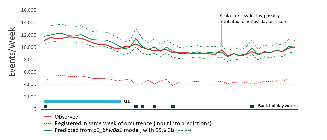
.xls .csvTo test whether 2019 showed a broadly similar delay profile as 2015 to 2018, the mean proportion of deaths occurred by weeks registration delay was examined for all data in the analysis (209 weeks combined for 2015 to 2018; 42 weeks combined for 2019). The mean proportion of deaths registered in the week of occurrence for the combined 2015 to 2018 years was 46.0%, compared with 47.0% for 2019. This may be because the period for registering 2019 deaths is shorter. Consequently, the model tends to over-estimate death occurrences (Figure 4).
The mean absolute model error for the 42 predictions based on 2019 data is 3.0% (on average the difference between predicted and observed deaths is 3.0% of the predicted value). The observed value was within the model predicted 95% confidence intervals for all 42 estimates.
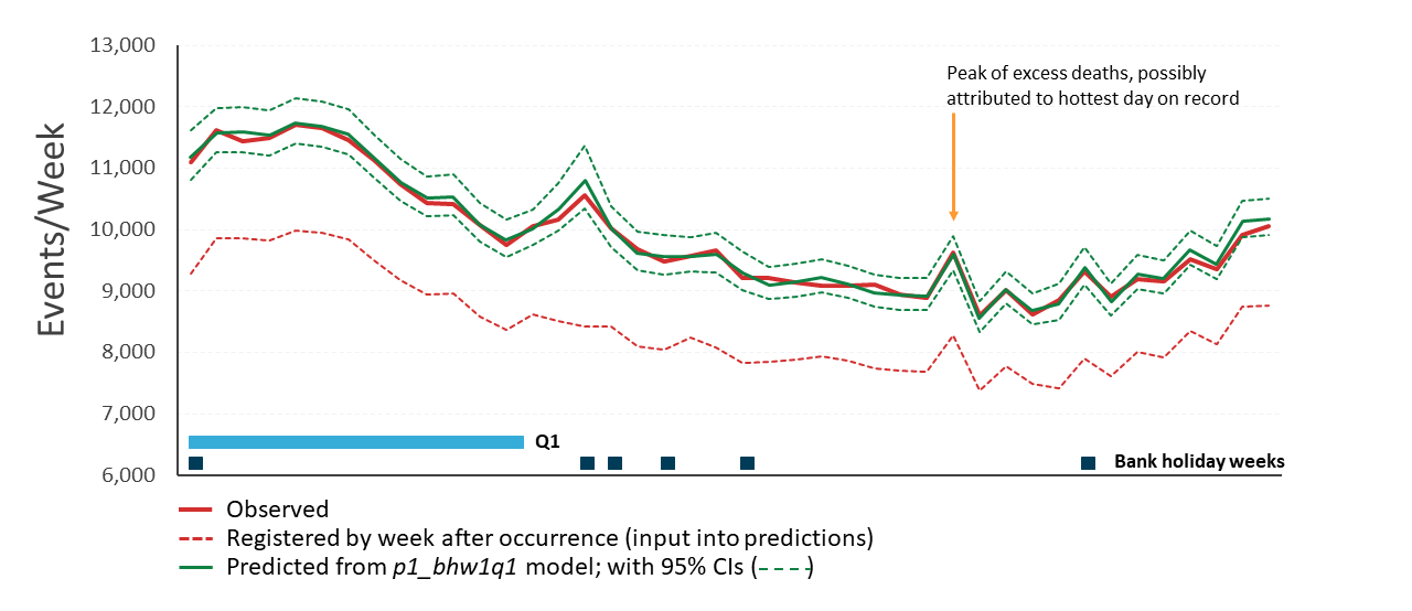
The observed occurrences show there to be around 600 to 800 excess deaths in week 30, compared with the trend. This week includes the hottest day on record, 25 July 2019. As there is no spike in registrations of deaths that occurred in week 30 in registration week 30, it is impossible to predict excess deaths from the registration data available in this same week (Figure 4).
Figure 4: The model predicted total deaths from registrations in the same week of occurrence is accurate but with low precision
Predicted occurrences based on numbers registered in the same week as occurrence from the p0_bhw0 model plotted against observed 2019 data for England and Wales (weeks 1 to 42). Wide 95% confidence intervals indicate low precision
Source: Office for National Statistics
Notes:
- Wide 95% confidence intervals indicate low precision.
Download this image Figure 4: The model predicted total deaths from registrations in the same week of occurrence is accurate but with low precision
.png (58.2 kB)
Expected proportion of deaths registered by the end of the week following occurrence (p1)
The effect of bank holidays on the proportion of deaths registered by the end of the week following occurrence is much stronger than the effect of Quarter 1 (Jan to Mar) (Tables 8 and 10, Appendix 2: Modelling registration delay). Consecutive bank holidays in the week of occurrence and the following week have the strongest effect (Table 3), followed by consecutive bank holidays in the two weeks following occurrence. In the absence of consecutive bank holidays, a bank holiday in either the week of occurrence or the following week has a significant effect.
The bank holiday and Quarter 1 effect are combined into a single model (called p1_bhw1q1) that is highly significant; approximately 61% of the weekly variation in the proportion of occurrences that are registered by the end of the week following occurrence (logit scale) is explained by the p1_bhw1q1 model (Table 11, Appendix 2: Modelling registration delay). The expected values derived from the p1_bhw1q1 model are shown in Table 3.
| Quarter (q1) | Bank holiday week category (bhw1) | Expected proportion of deaths registered | |
|---|---|---|---|
| Q2-4 | No bank holidays | 86.2% (83.5% - 88.5%) | |
| Q1 | No bank holidays | 85.1% (82.3% - 87.6%) | |
| Q2-4 | Bank holiday in occurrence and following week | 77.9% (74.1% - 81.3%) | |
| Q1 | Bank holiday in occurrence and following week | 76.4% (72.4% - 80.0%) | |
| Q2-4 | Bank holiday in occurrence or the following week | 84.2% (81.2% - 86.8%) | |
| Q1 | Bank holiday in occurrence or the following week | 83.0% (79.9% - 85.8%) | |
| Q2-4 | Consecutive bank holidays in the two week following occurrence | 82.4% (77.7% - 84.1%) | |
| Q1 | Consecutive bank holidays in the two weeks following occurrence | 81.1% (82.3% - 87.6%) |
Download this table Table 3: Deaths occurring in Quarter 1 (Jan to Mar) and weeks containing, or followed by weeks containing, bank holidays are expected to have lower rates of registration by the end of the following week
.xls .csvThe mean proportion of deaths registered by the end of the week following occurrence for the combined 2015 to 2018 years was 88.0%, compared with 88.5% for 2019. Again, this leads to a tendency for the model to over-estimate death occurrences (Figure 5). The mean absolute model error for the 42 predictions based on 2019 data is 0.7% and the observed value was within the model predicted 95% confidence intervals for all 42 estimates.
Figure 5: The model predicted total deaths from registrations by the end of the week following occurrence is both accurate and precise
Predicted occurrences based on numbers registered by the end of the week following occurrence from the p1_bhw1 model plotted against observed 2019 data for England and Wales (weeks 1 to 42)
Source: Office for National Statistics
Download this image Figure 5: The model predicted total deaths from registrations by the end of the week following occurrence is both accurate and precise
.png (76.1 kB)
Expected proportion of deaths registered by the end of the second week following occurrence (p2)
There is no significant difference between the proportion of deaths that are registered by the end of the second week after occurrence for Quarter 1 compared with other quarters (p=0.09). However, the bank holiday effect remains significant, though much less than in earlier models (Table 12, Appendix 2: Modelling registration delay).
The bank holiday effect has three categories, relating to whether there are zero, one or two weeks containing bank holidays in the week of occurrence and subsequent two weeks. The interaction of bank holidays with Quarter 1 is not significant and was dropped.
The final model called p2_bhw2 is significant and explains approximately 23% of the weekly variation in the proportion of occurrences that are registered by the end of the second week following occurrence (logit scale; Table 12, Appendix 2: Modelling registration delay). The expected values derived from the p2_bhw2 model are shown in Table 4.
| Bank Holiday week category (bhw2) | Expected proportion of deaths registered | |
|---|---|---|
| No Bank Holidays | 91.0% (89.6% - 92.1%) | |
| One Bank Holiday week in the occurrence or following two weeks | 90.5% (89.2% - 91.8%) | |
| Two Bank Holiday weeks in the occurrence and following two weeks | 89.6% (88.2% - 91.0%) |
Download this table Table 4: Deaths occurring in weeks containing, or followed by weeks containing, bank holidays are expected to have moderately lower rates of registration by the end of the second week
.xls .csvThe mean proportion of deaths registered by the end of the second week following occurrence for the combined 2015 to 2018 years was 90.7%, compared with 91.2% for 2019. Again, this leads to a tendency for the model to over-estimate death occurrences (Figure 6).
The analysis presented in Appendix 3 shows that the model performs poorly when assessed against week 37 and later for 2019 data. This is probably because the true number of occurrences is likely to be under-estimated by up to 2% (based on 98% of total deaths being registered by 26 weeks following occurrence). To week 36, there are no breaches of the model predicted total deaths 95% confidence intervals, but every week thereafter breaches. The mean absolute model error for the predictions based on 2019 data to week 36 is 0.4%.
Figure 6: The model predicted total deaths from registrations by the end of the second week following occurrence is accurate and very precise
Predicted occurrences based on numbers registered by the end of the second week following occurrence from the p2_bhw2 model plotted against observed 2019 data for England and Wales (weeks 1 to 36)
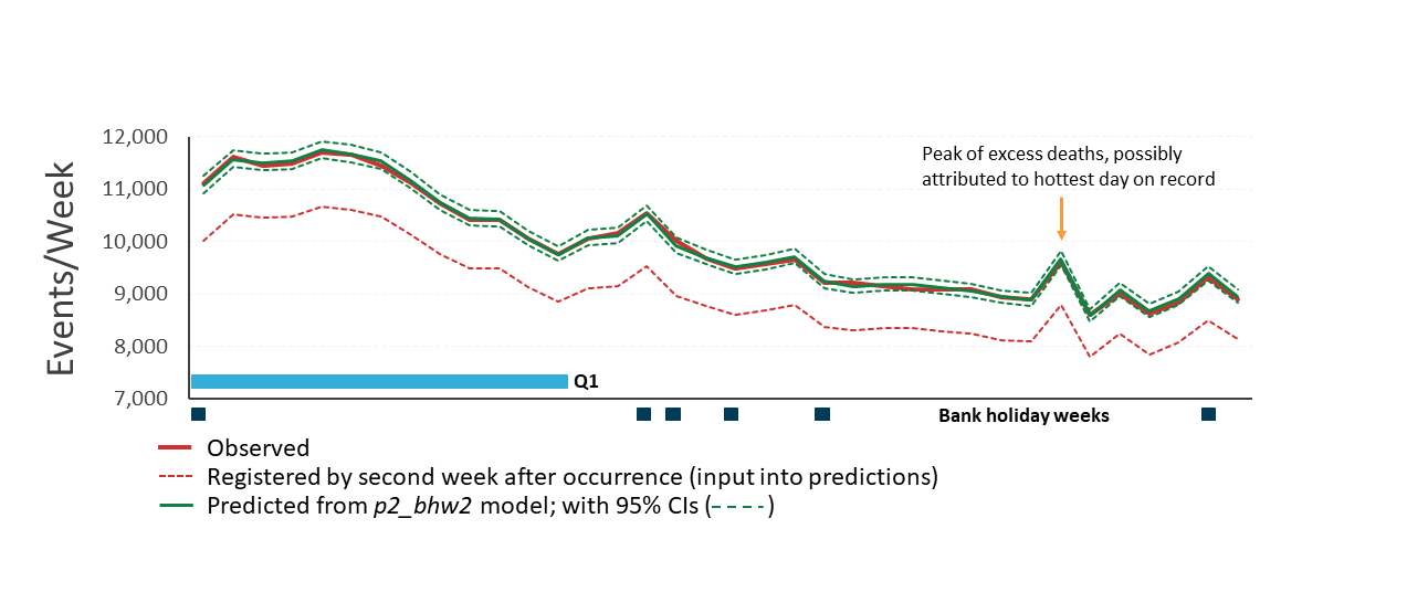
Source: Office for National Statistics
Download this image Figure 6: The model predicted total deaths from registrations by the end of the second week following occurrence is accurate and very precise
.png (63.5 kB)
The model accurately predicts excess deaths in week 30; a predicted 9,678 total deaths (confidence interval: 9,553 to 9,824) compared with the observed 9,625. The precision of the estimates is greater at the end of the second week following occurrence than a week earlier, but the accuracy shows little improvement.
The variation in the proportion of deaths registered at subsequent weeks following occurrence becomes less and though some effects remain significant, the expected proportions are all within 0.5% of each other. Should estimation beyond the second week after occurrence be required, it is proposed that the null model is used for predictions after a delay of two or more weeks (Table 1).
Back to table of contents5. Caveats of the approach
There are two large caveats with this approach. The first is that there is evidence that an increased number of deaths can itself add to registration delay (Appendix 1: Relationship between death registrations and death occurrences). If the primary purpose of this method is to estimate excess deaths, then this is compromised; the method is likely to under-estimate excess deaths (beyond what is captured by the winter, or Quarter 1 (Jan to Mar), effect).
Secondly, the method relies on the past being a reliable predictor of the future. Recent events following the coronavirus (COVID-19) pandemic have shown that extraordinary events can change registration behaviour. Registrations are currently happening over weekends and bank holidays at a rate they have not previously done and the level of control over the death registration process has relaxed. It is not clear to what extent these factors affect the modelling shown.
The models presented are based on weekly data and so can be limited by the day of week any bank holiday falls. An alternative approach is to model delay by day of occurrence and delay period in days or working days. Preliminary trials of such methods found that though the models fitted historic data closely, when they were used to predict total deaths it was found that there were many breaches of the confidence intervals produced by the model predictions by the observed data. We interpret this as over-fitting to the original data and moved to the methods described in this article.
Though less precise, we are satisfied that the confidence intervals produced by the weekly method are a greater reflection of the predictive power of the models compared with those built on daily data. We have shown that a week after the occurrence we can reliably predict total deaths from partial registration data with high accuracy and precision, using 2019 registration data.
Back to table of contents6. Appendix 1: Relationship between death registrations and death occurrences
The higher the number of occurrences, the lower the proportion of deaths that are registered in the same week as occurrence.
There are lower proportions of deaths registered in the same week as occurrence in Quarter 1 (Jan to Mar) compared with the summer (Figure 3). There is strong evidence that the number of weekly deaths strongly associates with Quarter 1 in 2018 (t test, p<0.001; Mean weekly deaths Q2-4 = 9,529 (± 1,195), Q1 (1) = 12,641 (± 1,760); see also Figure 7). This raises the question whether the Quarter 1 effect is a consequence of seasonal excess deaths. The Quarter 1 effect is highly significant in p0 models built with 2018 and with combined 2015 to 2018 data, but not significant using 2016 data (see Table 5). Quarter 1 of 2016 was mild and there were on average 1,277 extra deaths per week in Quarter 1 of 2016 compared with the rest of the year. In 2018, there were 3,111 extra deaths per week in Quarter 1 compared with the rest of the year.
The number of deaths correlates with the proportion of weekly deaths that were registered in the same week (Figure 7). The year 2016 had no weeks with over 12,000 deaths and the correlation between the number of occurrences and proportion of weekly deaths that were registered in the same week is weaker (Figure 7).
Figure 7: The number of death occurrences reduces the proportion that are registered within the same week
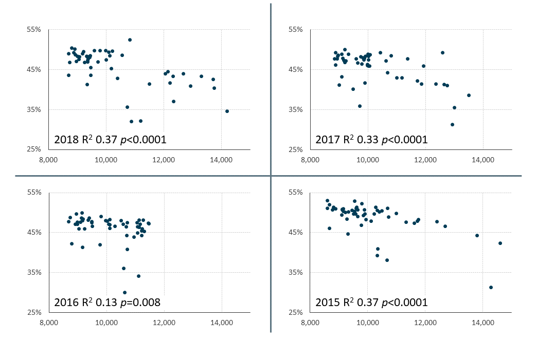
Notes:
- Data for England and Wales.
Download this image Figure 7: The number of death occurrences reduces the proportion that are registered within the same week
.png (47.4 kB)
7. Appendix 2: Modelling registration delay
The following equation is used to explore the relationship between explanatory factors and the proportion of deaths registered by time X:
logit pxi = βx0 + βx1 X1i + ... + βxn Xni
where:
- pxi is the proportion of deaths registered by time x for occurrence week i
- Xni is the value of the explanatory variable, Xn, for occurrence week i and βxn is the estimated size of the effect of Xn on logit px
- βx0 is the intercept
Null models are expressed as follows:
logit pxi = βx0
where the intercept βx0 is calculated as the mean logit pxi. These values were calculated and for p0 to p5 and presented in Table 1 (where p0 are the proportion of deaths that are registered in the same week that they occurred and p5 are the proportion of deaths that are registered by the end of the fifth subsequent week that they occurred).
An advantage of this formulation is that the variance is calculated as a single term. Models are built from two data sources: the single year’s data for 2018 and the combined data from 2015 to 2018. It is expected that models created from the combined data will be most robust, as single year effects are smoothed out.
An initial categorical variable called bhw_effect was created. This variable takes one of six values based on the proximity of bank holidays to the week of occurrence. In the 209 weeks of the combined dataset:
- 142 weeks take the value “No_BHW” as they do not occur within three weeks of a bank holiday
- 8 weeks take the value “OCCURRED_BHW_CONSEC” as the week of occurrence and the subsequent week both contain a bank holiday
- 20 weeks take the value “OCCURRED_ BHW” as the week of occurrence contains a bank holiday
- 12 weeks take the value “SUBSEQUENT_BHW” as the week subsequent to occurrence contains a bank holiday
- 8 weeks take the value “CONSECUTIVE_BHWs” as the week subsequent to occurrence and the following week both contain a bank holiday
- 19 weeks take the value “SECONDWEEK_BHW” as the second subsequent week to occurrence contains a bank holiday
A second categorical value, called Q1, is created. This defines the winter (Quarter 1) effect and when the week of the year is 1 to 13 it takes a value of 1 otherwise 0.
Estimating parameters of the expected proportion of occurrences that are registered in the same week (p0)
Estimation of the intercept (β00) from the null model (logit p0i = β00), based on data from 2018, is -0.1808 (Std Err, 0.0269) (Table 1; residual standard error 0.1941). Based on the combined data (2015 to 2018) the values are: β00 -0.1482 (Std Err, 0.0126); residual standard error 0.1825 [1/(1+exp(-β00))= 46.3%].
The winter effect (Q1) is examined first (Table 5). The expected proportion of deaths registered in the same week of occurrence in Quarter 1, based on combined 2015 to 2018 data, is 43.3% and 47.3% outside of Quarter 1 (Table 5).
| 2016 | 2018 | 2015 to 2018 | |||||||
|---|---|---|---|---|---|---|---|---|---|
| Est | Std Err | Pr | Est | Std Err | Pr | Est | Std Err | Pr | |
| Intercept | -0.1505 | 0.0275 | <0.001 | -0.1163 | 0.0256 | <0.001 | -0.1083 | 0.0135 | <0.001 |
| Q1 (1) | -0.0945 | 0.0556 | 0.0952 | -0.258 | 0.0511 | <0.001 | -0.1601 | 0.0271 | <0.001 |
| Residual | 0.1741 | F₁,₅₁ 2.9 | 0.1596 | F₁,₅₀ 25.5 | 0.1692 | F₁,₂₀₇ 35.0 | |||
| SSE/SST (R²) | 0.05 | 0.34 | 0.14 | ||||||
| E[p₀| Q1 (0)] | 46.2% (37.9% - 54.8%) | 47.1% (39.4% - 54.9%) | 47.3% (39.2% - 55.6%) | ||||||
| E[p₀ | Q1 (1)] | 43.9% (35.7% - 52.4%) | 40.8% (33.5% - 48.5%) | 43.3% (35.4% - 51.6%) | ||||||
Download this table Table 5: Quantification of the winter effect, Q1, upon the expected proportion of deaths registered in the same week as occurrence (p₀), England and Wales, 2015 to 2018
.xls .csvThe effect of bank holidays is examined next, using the variable bhw_effect described previously. When examining the impact of this variable upon the proportion of deaths that are registered in the same week as occurrence it is found that two categories are not significant (“CONSECUTIVE_BHWs” and “SECONDWEEK_BHW”) and a third, “SUBSEQUENT_BHW”, is only marginally significant (not shown). All these categories depend on bank holidays falling outside of the week of occurrence and not on those with bank holidays falling in the week of occurrence.
A second explanatory variable was constructed, bhw0, with just three categories:
- “OCCURRED_BHW_CONSEC” (Easter and Christmas, where the week of occurrence is followed by another bank holiday week)
- “OCCURRED_ BHW” (the remaining weeks of occurrence containing a bank holiday)
- “No_BHW”, the reference category
The expected proportion of deaths registered in the same week as occurrence is strongly affected by bank holidays in the week of occurrence and the subsequent week (Table 6). The effect is still strong, but not as severe, when there is a bank holiday in the week of occurrence but not the subsequent week.
| 2018 | 2015 to 2018 | ||||||
|---|---|---|---|---|---|---|---|
| Est | Std Err | Pr | Est | Std Err | Pr | ||
| Intercept | -0.1294 | 0.02 | <0.001 | -0.0977 | 0.0092 | <0.001 | |
| OCCURRED_BHW_CONSEC | -0.6188 | 0.0969 | <0.001 | -0.5541 | 0.0445 | <0.001 | |
| OCCURRED_BHW | -0.2876 | 0.0632 | <0.001 | -0.3061 | 0.0291 | <0.001 | |
| Residual | 0.134 | F₂,₄₉ 29.0 | 0.1233 | F₂,₂₀₆ 124.9 | |||
| SSE/SST (R²) | 0.54 | 0.55 | |||||
| E[p₀ | No_BHW ] | 46.8% (40.3% - 53.3%) | 47.6% (41.6% - 53.6%) | |||||
| E[p₀ | OCCURRED_BHW_CONSEC ] | 32.1% (26.7% - 38.1%) | 34.3% (29.0% - 39.9%) | |||||
| E[p₀| OCCURRED_BHW ] | 39.7% (33.6% - 46.2%) | 40.0% (34.4% - 46.0%) | |||||
Download this table Table 6: Quantification of the bank holiday effect, bhw0, upon the expected proportion of deaths registered in the same week as occurrence (p<sub>0</sub>), England and Wales, 2015 to 2018
.xls .csvThe two effects were combined into a single model (called p0_bhw0q1) that marks a significant improvement in model fit (Table 7). Between 71% and 82% of the weekly variation in the proportion of occurrences that are registered in the same week as occurrence is explained by the p0_bhw0q1 model (Table 7; SSE/SST (R2), logit scale).
| 2018 | 2015 to 2018 | ||||||
|---|---|---|---|---|---|---|---|
| Est | Std Err | Pr | Est | Std Err | Pr | ||
| Intercept | -0.0714 | 0.0142 | <0.001 | -0.0550 | 0.0084 | <0.001 | |
| OCCURRED_BHW_CONSEC | -0.5582 | 0.0613 | <0.001 | -0.5548 | 0.0360 | <0.001 | |
| OCCURRED_BHW | -0.2891 | 0.0397 | <0.001 | -0.3152 | 0.0235 | <0.001 | |
| Q1 (1) | -0.2370 | 0.0272 | <0.001 | <0.001 | |||
| Residual | 0.0842 | F₃,₄₈ 74.3 | 0.0996 | F₃,₂₀₅ 164.5 | |||
| SSE/SST (R²) | 0.82 | 0.71 | |||||
Download this table Table 7: Parameterisation of p0_bhw0q1 models that utilise bhw0 and Q1 as explanatory factors to estimate the expected proportion of deaths registered in the same week as occurrence, England and Wales, 2015 to 2018
.xls .csvEstimating parameters of the expected proportion of occurrences that are registered by the end of the subsequent week (p1)
Estimation of the intercept (β<10) from the null model (logit p1i = β10), based on data from 2018, is 1.6949 (Std Err, 0.0210) (Table 1; residual standard error 0.1500). Based on the combined data (2015-2018) the values are: β10 1.7544 (Std Err, 0.0118); residual standard error 0.1700 [1/(1+exp(-β10)) = 85.3%].
The winter effect is much weaker in explaining variation in the proportion of occurrences that are registered by the end of the subsequent week (p1), compared with in the same week (p0). The winter effect is significant in 2018 but only marginally when combined 2015 to 2018 data are examined (Table 8).
| 2018 | 2015 to 2018 | ||||||
|---|---|---|---|---|---|---|---|
| Est | Std Err | Pr | Est | Std Err | Pr | ||
| Intercept | 1.7366 | 0.0212 | <0.001 | 1.7741 | 0.0133 | <0.001 | |
| Q1 (1) | -0.1666 | 0.0424 | <0.001 | -0.0792 | 0.0266 | 0.003 | |
| Residual | 0.1324 | F₁,₅₀ 15.4 | 0.1664 | F₁,₂₀₇ 8.8 | |||
| SSE/SST (R²) | 0.24 | 0.04 | |||||
| E[p₁ | Q1 (0)] | 85.0% (81.4% - 88.0%) | 85.5% (81.0% - 89.1%) | |||||
| E[p₁ | Q1 (1)] | 82.8% (78.8% - 86.2%) | 84.5% (79.7% - 88.3%) | |||||
Download this table Table 8: Quantification of the winter effect, Q1, upon the expected proportion of deaths registered by the end of the week following occurrence (p₁), England and Wales, 2015 to 2018
.xls .csvThe effect of bank holidays upon the proportion of deaths that are registered by the end of the week subsequent to occurrence was examined using bhw_effect. The “SECONDWEEK_BHW” category, which relates to the presence of a bank holiday in the second week after occurrence, was not significant in models explaining the proportion of deaths that are registered by the end of the week subsequent to occurrence. A second explanatory variable was constructed, bhw1_1, that merges the “SECONDWEEK_BHW” into the reference category “No_BHW”.
This five-category variable, bhw1_1, explains about the same proportion of variation in the proportion of deaths that are registered by the end of the week subsequent to occurrence as the three-category variable, bhw0, did for variation in the proportion of deaths that are registered in the same week as occurrence (combined 2015 to 2018 data: Table 9, 56%; compared with Table 6, 55%).
| 2018 | 2015 to 2018 | ||||||
|---|---|---|---|---|---|---|---|
| Est | Std Err | Pr | Est | Std Err | Pr | ||
| Intercept | 1.7491 | 0.0146 | <0.001 | 1.8099 | 0.0089 | <0.001 | |
| OCCURRED_BHW_CONSEC | -0.5103 | 0.0668 | <0.001 | -0.5707 | 0.0411 | <0.001 | |
| OCCURRED_BHW | -0.1407 | 0.0438 | 0.002 | -0.1356 | 0.0269 | <0.001 | |
| SUBSEQUENT_BHW | -0.1438 | 0.0552 | 0.012 | -0.1619 | 0.034 | <0.001 | |
| CONSECUTIVE_BHWs | -0.3299 | 0.0668 | <0.001 | -0.2973 | 0.0411 | <0.001 | |
| Residual | 0.0923 | F₄,₄₇ 21.9 | 0.1135 | F₄,₂₀₄ 65.0 | |||
| SSE/SST (R²) | 0.65 | 0.56 | |||||
| E[p₁ | No_BHW ] | 85.2% (82.8% - 87.3%) | 85.9% (83.0% - 88.4%) | |||||
| E[p₁ | OCCURRED_BHW_CONSEC ] | 77.5% (74.2% - 80.5%) | 77.5% (73.4% - 81.2%) | |||||
| E[p₁| OCCURRED_BHW ] | 83.3% (80.7% - 85.7%) | 84.2% (81.0% - 87.0%) | |||||
| E[p₁ | SUBSEQUENT_BHW ] | 83.3% (80.6% - 85.6%) | 83.9% (80.6% - 86.7%) | |||||
| E[p₁ | CONSECUTIVE_BHWs ] | 80.5% (77.5% - 83.2%) | 81.9% (78.4% - 85.0%) | |||||
Download this table Table 9: Quantification of the bank holiday effect, bhw1_1, upon the expected proportion of deaths registered by the end of the week following occurrence (p₁), England and Wales, 2015 to 2018
.xls .csvThe categories “OCCURRED_ BHW” and “SUBSEQUENT_BHW” relate to the week of occurrence containing a bank holiday or the week after, respectively. Based on visual examination of Figure 3, it was expected that the category “SUBSEQUENT_BHW” would have a stronger effect than “OCCURRED_ BHW”. However, they have an almost identical effect upon the proportion of occurrences registered by the end of the subsequent week (Table 9) and the categories are combined to create a new category, called “OCCURRED_ or_SUBSEQUENT”, in bhw1 (Table 10). The revised variable, bhw1, performs better than bhw1_1, and is used going forwards (Table 10).
| 2018 | 2015 to 2018 | ||||||
|---|---|---|---|---|---|---|---|
| Est | Std Err | Pr | Est | Std Err | Pr | ||
| Intercept | 1.7491 | 0.0144 | <0.001 | 1.8099 | 0.0089 | <0.001 | |
| OCCURRED_BHW_CONSEC | -0.5103 | 0.0661 | <0.001 | -0.5707 | 0.0411 | <0.001 | |
| OCCURRED_or_SUBSEQUENT | -0.1418 | 0.0354 | <0.001 | -0.1455 | 0.0219 | <0.001 | |
| CONSECUTIVE_BHWs | -0.3299 | 0.0661 | <0.001 | -0.2973 | 0.0411 | <0.001 | |
| Residual | 0.0913 | F₁,₄₈ 29.9 | 0.1133 | F₁,₂₀₅ 86.8 | |||
| SSE/SST (R²) | 0.65 | 0.56 | |||||
| E[p₁ | No_BHW ] | 85.2% (82.8% - 87.3%) | 85.9% (83.0% - 88.4%) | |||||
| E[p₁ | OCCURRED_BHW_CONSEC] | 77.5% (74.3% - 80.5%) | 77.5% (73.4% - 81.2%) | |||||
| E[p₁ | OCCURRED_or_SUBSEQUENT] | 83.3% (80.7% - 85.6%) | 84.1% (80.9% - 86.8%) | |||||
| E[p₁ | CONSECUTIVE_BHWs] | 80.5% (77.6% - 83.2%) | 81.9% (78.4% - 85.0%) | |||||
Download this table Table 10: Quantification of the bank holiday effect, bhw1, upon the expected proportion of deaths registered by the end of the week following occurrence (p₁), England and Wales, 2015 to 2018
.xls .csvThe two effects were combined into a single model (called p1_bhw1q1) that marks a significant improvement in model fit (Table 11). Between 61% and 82% of the weekly variation in the proportion of occurrences that are registered by the end of the week subsequent to occurrence is explained by the p1_bhw1q1 model (Table 11; SSE/SST (R2), logit scale).
| 2018 | 2015 to 2018 | ||||||
|---|---|---|---|---|---|---|---|
| Est | Std Err | Pr | Est | Std Err | Pr | ||
| Intercept | 1.785 | 0.0118 | <0.001 | 1.8333 | 0.0096 | <0.001 | |
| OCCURRED_BHW_CONSEC | -0.4744 | 0.0484 | <0.001 | -0.5722 | 0.0388 | <0.001 | |
| OCCURRED_or_SUBSEQUENT | -0.1598 | 0.0258 | <0.001 | -0.1579 | 0.0209 | <0.001 | |
| CONSECUTIVE_BHWs | -0.294 | 0.0484 | <0.001 | -0.2878 | 0.0388 | <0.001 | |
| Q1 (1) | -0.1436 | 0.0217 | <0.001 | -0.0876 | 0.0173 | <0.001 | |
| Residual | 0.0663 | F₄,₄₇ 53.4 | 0.1071 | F₄,₂₀₄ 79.4 | |||
| SSE/SST (R²) | 0.82 | 0.61 | |||||
Download this table Table 11: Parameterisation of p1_bhw1q1 models that use bhw1 and Q1 as explanatory factors to estimate the expected proportion of deaths registered by the end of the week subsequent to occurrence,
.xls .csvEstimating parameters of the expected proportion of occurrences that are registered by the end of the second week after occurrence (p2)
Estimation of the intercept (β20) from the null model (logit p2i = β20), based on data from 2018, is 2.2506 (Std Err, 0.0098) (Table 1; residual standard error 0.0703). Based on the combined data (2015 to 2018) the values are: β20 2.2846 (Std Err, 0.0061); residual standard error 0.0873 [1/(1+exp(-β20)) = 90.8%].
The total variation (SST) in the 2015 to 2018 derived null models has fallen from 6.9302 (p0) through 5.9798 (p1) to 1.5854 for the proportion (logit scale) of occurrences that are registered by the end of the second week after occurrence (p2). So by the end of the second week after occurrence there is much less variation to explain and the null model may be sufficient for our needs.
The bank holiday effect remains significant, though much less than in earlier models (F5,203 12.7. The categories “OCCURRED_ BHW”, “SUBSEQUENT_BHW” and “SECONDWEEK_BHW” all relate to containing a single week with bank holidays out of the three-week period. They had identical effects and are combined to create a new category, called “SINGLE_BHW”, in bhw2.
Similarly, the categories “OCCURRED_BHW_CONSECUTIVE_BHWs” and “CONSECUTIVE_BHWs” relate to containing two consecutive weeks with bank holidays out of the three-week period. These too had identical effects and are combined to create a new category, called “TWO_BHWs”, in bhw2. This variable has three categories, with “No_BHW” being the reference category. The impact of bhw2 on explaining variation in the proportion of occurrences that are registered by the end of the second week after occurrence is investigated in Table 12.
| 2018 | 2015 to 2018 | ||||||
|---|---|---|---|---|---|---|---|
| Est | Std Err | Pr | Est | Std Err | Pr | ||
| Intercept | 2.2759 | 0.0096 | <0.001 | 2.3081 | 0.0064 | <0.001 | |
| TWO_BHWs | -0.1476 | 0.0299 | <0.001 | -0.1506 | 0.0203 | <0.001 | |
| SINGLE_BHW | -0.0559 | 0.0184 | 0.004 | -0.049 | 0.0125 | <0.001 | |
| Residual | 0.0567 | F₂,₄₉ 14.7 | 0.0768 | F₂,₂₀₆ 31.4 | |||
| SSE/SST (R²) | 0.37 | 0.23 | |||||
Download this table Table 12: Quantification of the bank holiday effect, bhw2, upon the expected proportion of deaths registered by the end of the second week after occurrence (p₂), England and Wales, 2015 to 2018
.xls .csv8. Appendix 3: Measuring performance against 2019 data
To test whether 2019 showed a broadly similar delay profile as 2015 to 2018, the mean proportion of deaths occurred by weeks registration delay was examined for all data in the analysis (209 weeks combined for 2015 to 2018; 42 weeks combined for 2019). The mean proportion of deaths registered by weeks since occurrence tended to be higher in 2019 than in the combined 2015 to 2018 data (Table 13). A caveat of this analysis is that part of this may because the period for registering 2019 deaths is shorter.
| Registration delay (weeks since occurrence) | ||||||||||
|---|---|---|---|---|---|---|---|---|---|---|
| Year | 0 | 1 | 2 | 3 | 4 | 5 | 10 | 15 | 20 | 25 |
| 2019 | 47.0% | 85.5% | 91.2% | 92.5% | 93.1% | 93.5% | 94.8% | 96.0% | 96.9% | 97.7% |
| 2015 to 2018 | 46.0% | 85.0% | 90.7% | 92.0% | 92.5% | 92.9% | 94.3% | 95.6% | 96.8% | 97.7% |
Download this table Table 13: A greater proportion of deaths tended to be registered by each weeks’ delay in 2019 than in 2015 to 2018, England and Wales
.xls .csvModel assessment is presented graphically and is based on analysis of variance of model predicted registration rates against those observed (SSEmodel/SST), the mean absolute error (proportion of the expected count) and the number of breaches of the 42 observed values over 95% confidence intervals.
The predicted number of occurrences is based on the estimated proportion registered by time x, px. The number of registrations observed by time x (Robsx) is multiplied by the reciprocal of px, such that Predicted = (Robsx)/px. Error in predictions is given as a proportion of expected values.
Performance of models based on the number registered in the same week as occurrence (p0)
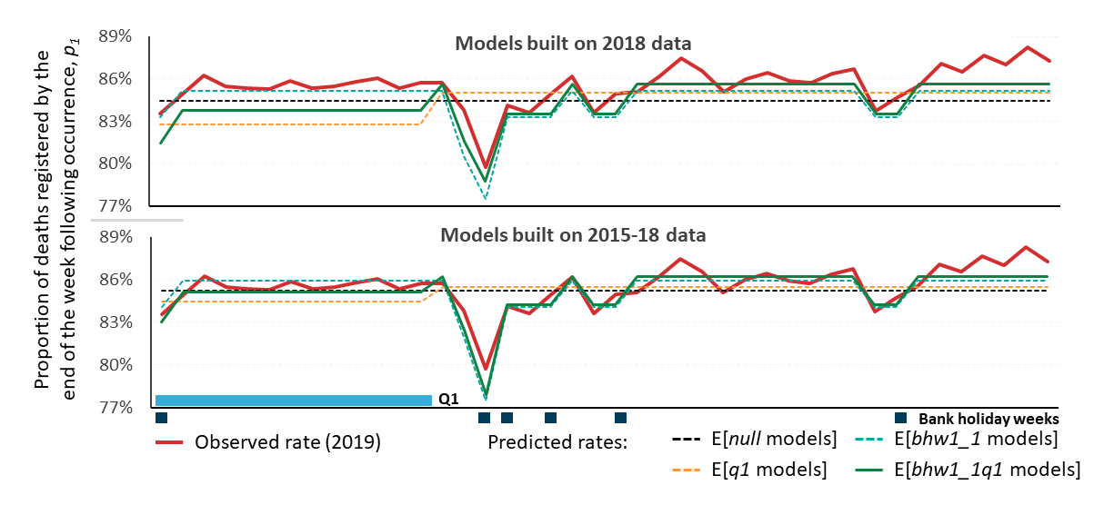
All models tend to under-estimate the proportion registered in the same week of occurrence (Figure 8). In all cases, the 2015 to 2018 models perform better than the 2018 model (Table 14). The p0_bhw0q1 and p0_bhw0 models perform best (Table 14).
Figure 8: Expected proportions of deaths that are registered in the same week as occurrence based on models built on 2018 and 2015-2018 data plotted against the observed 2019 data
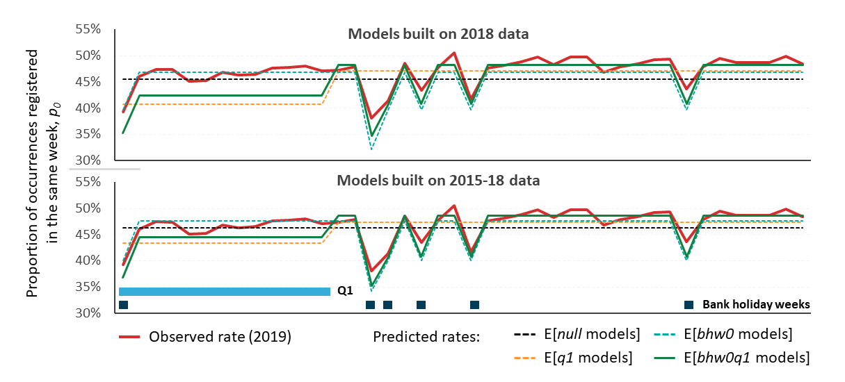
Source: Office for National Statistics
Download this image Figure 8: Expected proportions of deaths that are registered in the same week as occurrence based on models built on 2018 and 2015-2018 data plotted against the observed 2019 data
.png (80.3 kB)
| 2018 | 2015 to 2018 | ||||||
|---|---|---|---|---|---|---|---|
| SSE/SST | Mean |error| | Breaches | SSE/SST | Mean |error| | Breaches | ||
| p0_null | 0 | 6.0% | 0 | 0 | 5.1% | 0 | |
| p0_q1 | 0.043 | 7.2% | 1 | 0.043 | 5.6% | 1 | |
| p0_bhw0 | 0.766 | 3.7% | 1 | 0.777 | 2.8% | 0 | |
| p0_bhw0q1 | 0.733 | 4.5% | 9 | 0.844 | 3.0% | 0 | |
Download this table Table 14: Accuracy of the p0 models to predict total death occurrences from the number of registrations that occur in the same week as death occurrence in 2019
.xls .csvPerformance of models based on the number registered by the end of the week following occurrence (p1)
All models tend to under-estimate the proportion registered in the same week of occurrence (Figure 9), but care should be taken interpreting data relating to late 2019 as the true number of occurrences is likely to be under-estimated by 2% (Table 13) leading to a higher than actual proportion of deaths registered by the end of the week following occurrence. In all cases, the 2015 to 2018 models perform better than the 2018 models and p1_bhw1q1 and p1_bhw1 models perform best (Table 15).
Figure 9: Expected proportions of deaths that are registered by the end of the week following occurrence based on models built on 2018 and 2015-2018 data plotted against the observed 2019 data
Source: Office for National Statistics
Download this image Figure 9: Expected proportions of deaths that are registered by the end of the week following occurrence based on models built on 2018 and 2015-2018 data plotted against the observed 2019 data
.png (76.2 kB)
| 2018 | 2015 to 2018 | ||||||
|---|---|---|---|---|---|---|---|
| SSE/SST | Mean |error| | Breaches | SSE/SST | Mean |error| | Breaches | ||
| p1_null | 0 | 1.7% | 2 | 0 | 1.2% | 1 | |
| p1_q1 | 0.003 | 2.1% | 3 | 0.003 | 1.4% | 1 | |
| p1_bhw1 | 0.689 | 1.2% | 4 | 0.701 | 0.8% | 0 | |
| p1_ bhw1q1 | 0.707 | 1.4% | 13 | 0.776 | 0.7% | 0 | |
Download this table Table 15: Accuracy of the p1 models to predict total death occurrences from the number of deaths registered by the end of the week following occurrence in 2019.
.xls .csvPerformance of models based on the number registered by the end of the second week following occurrence (p2)
From 37 weeks, the observed proportions registered are out of line with historical observations and their derived models (Figure 10). Evaluation is therefore based on the first 36 weeks of 2019 (Table 16). To week 36, there are no breaches of the model predicted total deaths 95% confidence intervals, but every week thereafter breaches. The mean absolute model error for the predictions based on 2019 data to week 36 is 0.4%.
Figure 10: Expected proportions of deaths that are registered by the end of the second week following occurrence based on models built on 2018 and 2015-2018 data plotted against the observed 2019 data

Source: Office for National Statistics
Download this image Figure 10: Expected proportions of deaths that are registered by the end of the second week following occurrence based on models built on 2018 and 2015-2018 data plotted against the observed 2019 data
.png (39.6 kB)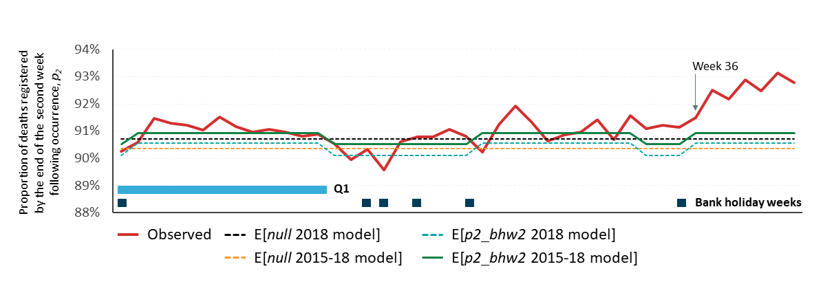
| 2018 | 2015-18 | ||||||
|---|---|---|---|---|---|---|---|
| SSE/SST | Mean |error| | Breaches | SSE/SST | Mean |error| | Breaches | ||
| p2_null | 0 | 0.7% | 4 | 0 | 0.7% | 0 | |
| p2_ bhw2 | 0.234 | 0.5% | 9 | 0.234 | 0.4% | 0 | |