1. Main points
In July 2012 to June 2014:
Aggregate total wealth of all private households in Great Britain was £11.1 trillion
The wealthiest 10% of households owned 45% of total aggregate household wealth
The least wealthy half of households owned 9% of total aggregate household wealth
Private pension wealth was the largest component of aggregate total wealth
Half of all households had total wealth of £225,100 or more
Households in the South East had the highest median wealth (£342,400)
2. Introduction
This chapter looks at total net wealth of private households in Great Britain. The definition of wealth used in this survey is an economic one: total wealth (gross) is the value of accumulated assets, and total wealth (net) is the value of accumulated assets minus the value of accumulated liabilities.
Total net wealth is defined as the sum of 4 components1: property wealth (net), physical wealth, financial wealth (net) and private pension wealth. It does not include business assets owned by household members, for instance if they run a business; nor does it include rights to state pensions, which people accrue during their working lives and draw on in retirement.
Net wealth is a ‘stock’ concept rather than a ‘flow’ concept. In other words, it refers to the balance at a point in time. In contrast, income refers to the flow of resources over time. Income allows the wealth to be accumulated, but equally, wealth is capable of producing flows of income either in the present or – as in the case of pension wealth – in the future.
All estimates are presented as current values (that is, the value at time of interview) and have not been adjusted for inflation.
Due to the complexity of the data, for example, the use of imputed values and complex weighting, only a very limited amount of high level significance testing has been undertaken, which is presented in the Technical chapter of this report (335.5 Kb Pdf). None of the estimates commented on in this chapter have been tested for significance.
Notes for Introduction:
Back to table of contents3. Aggregate total wealth
Aggregate total wealth (including private pension wealth) of all private households in Great Britain was £11.1 trillion in the period July 2012 to June 2014, an 18% increase from the previous period of July 2010 to June 2012 (Table 2.1).
Table 2.1: Breakdown of aggregate total wealth, by components
| Great Britain, July 2006 to June 2014 | ||||
| £ Billion | ||||
| July 2012 to June 2014 | July 2010 to June 2012 | July 2008 to June 2010 | July 2006 to June 20081 | |
| Property Wealth (net) | 3,927 | 3,528 | 3,379 | 3,537 |
| Financial Wealth (net) | 1,596 | 1,305 | 1,091 | 1,043 |
| Physical Wealth1 | 1,152 | 1,081 | 1,016 | 961 |
| Private Pension Wealth | 4,459 | 3,530 | 3,470 | 2,886 |
| Total Wealth (including Private Pension Wealth)1 | 11,134 | 9,444 | 8,955 | 8,426 |
| Total Wealth (excluding Private Pension Wealth)1 | 6,676 | 5,914 | 5,485 | 5,540 |
| Source: Office for National Statistics | ||||
| Notes: | ||||
| 1. July 2006 to June 2008 estimates for physical and total wealth are based on half sample. | ||||
Download this table Table 2.1: Breakdown of aggregate total wealth, by components
.xls (25.1 kB)Figure 2.2 shows the relative contribution of each of the 4 wealth components to aggregate total wealth. The 2 components making the largest contribution to aggregate total wealth were private pension wealth and net property wealth (accounting for 40% and 35% respectively in the period July 2012 to June 2014). Financial wealth made up 14% of the total wealth in this period and physical wealth made the smallest contribution of the 4 components (10%).
Figure 2.2: Breakdown of aggregate total wealth, by components
Great Britain, July 2010 to June 2014
Source: Wealth and Assets Survey - Office for National Statistics
Download this chart Figure 2.2: Breakdown of aggregate total wealth, by components
Image .csv .xlsThe impact of private pension wealth
Chapter 6 of this publication considers the value of private pension wealth. The methodology used to calculate the value of private pensions is complicated and represents a person’s future pension retirement expressed as an equivalent ‘pot of money’. There are a number of different types of pensions and a slightly different valuation method applied to each. The value of some types of pensions (defined benefit (DB) type pensions) is calculated using financial assumptions (discount rates and annuity factors) which change over time. These external factors can ‘cause’ changes, for example, an individual may be paying exactly the same amount of money into a pension at 2 points in time but the value of the pension pot they have accumulated will have changed due to the annuity rates and discount factors prevailing at the time.
If the relative contribution to total wealth is considered excluding private pension wealth, the pattern of change for the remaining types of wealth is a little clearer. Property wealth accounted for 59% of total wealth (excluding private pension wealth) in July 2012 to June 2014. This has been consistently falling over the 4 survey periods to date, from a high of 64% in July 2006 to June 2008. Financial wealth accounted for 24% of total wealth (excluding private pension wealth) in July 2012 to June 2014. This has been consistently rising over the 4 survey periods to date, from a low of 19% in July 2006 to June 2008. Physical wealth accounted for 17% of total wealth (excluding private pension wealth) in July 2012 to June 2014. The contribution of physical wealth fluctuates more over time but only by 1% or 2%.
Back to table of contents4. Distribution of aggregate total wealth
This section explores a number of different ways of considering the distribution or inequality of wealth.
Figure 2.3 shows aggregate total wealth (including private pension wealth) by deciles and the breakdown of each decile into its components. Deciles divide the data, sorted in ascending order, into ten equal parts so that each part contains 10% (or one-tenth) of the wealth distribution – from the least wealthy households in the first decile to the wealthiest in the 10th decile.
The wealthiest 10% of households owned 45% of aggregate total wealth in July 2012 to June 2014. The wealthiest 10% of households were 2.4 times wealthier than the second wealthiest 10% – this has been consistent across all 4 survey periods. In July 2012 to June 2014, the wealthiest 10% of households were 5.2 times wealthier than the bottom 50% of households (the bottom 5 deciles combined). The bottom 50% of households owned 9% of aggregate total wealth. (See Chapter 7 – Extended Analyses)
By combining the top 2 deciles and the bottom 2 deciles, a comparison can be made between the value of aggregate total wealth for the wealthiest 20% of private households within Great Britain and the least wealthy 20%. In July 2012 to June 2014, the wealthiest 20% of households had 117 times more aggregate total wealth than the least wealthy 20% of households. In comparison, the wealthiest 20% of households had 97 times more aggregate total wealth than the least wealthy 20% of households in July 2010 to June 2012.
The wealthiest 20% of households owned 64% of total aggregate household wealth in July 2012 to June 2014; a share which has increased slightly from 62% in the 3 previous survey periods.
Figure 2.3: Breakdown of aggregate total wealth, by deciles and components
Great Britain, July 2012 to June 2014
Source: Wealth and Assets Survey - Office for National Statistics
Download this chart Figure 2.3: Breakdown of aggregate total wealth, by deciles and components
Image .csv .xlsIn the period July 2012 to June 2014, physical wealth made the largest contribution to aggregate total wealth for households in the lowest 3 deciles. Net property wealth made the largest contribution towards aggregate total wealth for households in the fourth through to the eighth deciles. Private pension wealth made the largest contribution to aggregate total wealth for households in the top 2 wealth deciles.
Figure 2.4 illustrates the breakdown of aggregate total wealth for the lowest 3 deciles in more detail. The first thing to note is that the bar for the lowest decile straddles the x-axis. This highlights the fact that the sums of certain wealth components are negative for this group.
Considering the bottom 10% of households, physical wealth made the largest positive contribution to the aggregate wealth value, with a smaller positive contribution being made by private pension wealth. Both the aggregate values of net financial wealth and net property wealth were negative. This does not imply that all households in this least wealthy group would necessarily have no property wealth (for example, rent their home), have negative property wealth (that is, the debt on their property outweighs its value) or have negative financial wealth; this would depend on their overall total wealth. For example, a household with heavy debts could still fall into this group even if they were property owners. However, it is likely that many in this lowest 10% would be those with no property wealth, negative property wealth or notable financial liabilities. Amongst the second and third wealth deciles, all components of wealth were positive, with physical wealth again making the largest contribution.
Figure 2.4: Breakdown of aggregate total wealth, by lowest 3 deciles and components
Great Britain, July 2012 to June 2014
Source: Wealth and Assets Survey - Office for National Statistics
Download this chart Figure 2.4: Breakdown of aggregate total wealth, by lowest 3 deciles and components
Image .csv .xlsThe distributions of the different components of aggregate total wealth can be compared by calculating Gini coefficients. The Gini coefficient takes a value between 0 and 1, with 0 representing a perfectly equal distribution and 1 representing maximal inequality.
Table 2.5: Gini Coefficients for aggregate total wealth, by components
| Great Britain, July 2006 to June 2014 | ||||
| Gini Coefficient | ||||
| July 2012 to June 2014 | July 2010 to June 2012 | July 2008 to June 2010 | July 2006 to June 20081 | |
| Property Wealth (net) | 0.66 | 0.64 | 0.63 | 0.63 |
| Financial Wealth (net) | 0.91 | 0.92 | 0.89 | 0.89 |
| Physical Wealth1 | 0.45 | 0.44 | 0.45 | 0.46 |
| Private Pension Wealth | 0.73 | 0.73 | 0.76 | 0.77 |
| Total Wealth1 | 0.63 | 0.61 | 0.61 | 0.61 |
| Source: Wealth and Assets Survey, Office for National Statistics | ||||
| Notes: | ||||
| 1. July 2006 to June 2008 estimates for physical and total wealth are based on half sample. | ||||
Download this table Table 2.5: Gini Coefficients for aggregate total wealth, by components
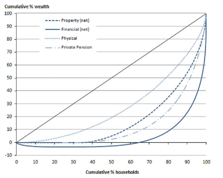
.xls (25.6 kB)Of the 4 wealth components, inequality remains lowest for physical wealth, with a Gini coefficient 0.45 in the period July 2012 to June 2014. Unlike the other wealth components, every household has some physical assets (that is, a positive wealth value). Inequality remains highest for the net financial wealth component, with a Gini coefficient 0.91 in the period July 2012 to June 2014. However, although the order in which the 4 components display inequality remains the same, inequality has consistently worsened for property wealth (that is, the Gini coefficients have increased slightly over time) over the 4 survey periods.
Figure 2.6: Lorenz curves for the components of wealth
Great Britain, July 2012 to June 2014
Source: Wealth and Assets Survey - Office for National Statistics
Download this image Figure 2.6: Lorenz curves for the components of wealth
.png (105.1 kB) .xls (1.9 MB)
The difference in inequality between each of the 4 wealth components is illustrated in Figure 2.6, which shows the Lorenz curves1 for the wealth components in the period July 2012 to June 2014. Lorenz curves are a graphical representation of the inequality of distribution; where the diagonal 45 degree line illustrates a scenario where wealth is equally shared. The closer the Lorenz curve is to the diagonal line, the more equal the distribution becomes. The most inequality is in net financial wealth, whilst physical wealth shows the most equality. The curves for net financial wealth and net property wealth hold negative values of cumulative wealth. This is because some households have negative net wealth for these particular components.
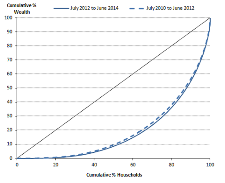
Figure 2.7 plots the Lorenz curve for total aggregate wealth in the period July 2012 to June 2014 and the previous period of July 2010 to June 2012. Since there was so little difference in the distribution of aggregate total wealth between the waves, the curves for the first 2 waves have not been included. This indicates that inequality has worsened slightly overall between the last 2 survey periods (also seen in the increase in the Gini coefficient for total wealth in Table 2.5).
Figure 2.7: Lorenz curves for aggregate total wealth including private pension wealth
Great Britain, July 2010 to June
Source: Wealth and Assets Survey - Office for National Statistics
Download this image Figure 2.7: Lorenz curves for aggregate total wealth including private pension wealth
.png (72.8 kB) .xls (2.1 MB)
Notes for distribution of aggregate total wealth
A Lorenz curve is created by ranking households from poorest to richest and graphing the cumulative share of household income and households as a proportion of total income and households respectively.
The breaks are fairly arbitrary, but have been chosen to give a reasonably balanced distribution across all households. Note that the lowest band of household total wealth (<£20,000) will include some households with negative total wealth.
5. Household total wealth
In the next section, total household wealth is considered. This is a net wealth measure for each household created by adding together the different components of household wealth: property wealth (net), financial wealth (net), physical wealth and private pension wealth.
Table 2.8: Median household total wealth
| Great Britain, July 2006 to June 2014 | ||||
| £ | ||||
| July 2012 to June 2014 | July 2010 to June 2012 | July 2008 to June 2010 | July 2006 to June 20081 | |
| Median household wealth including pension wealth | 225,100 | 216,500 | 204,300 | 196,700 |
| Median household wealth excluding pension wealth | 141,400 | 145,600 | 144,500 | 146,600 |
| Source: Wealth and Assets Survey, Office for National Statistics | ||||
| Notes: | ||||
| 1. July 2006 to June 2008 estimates are based on half sample. | ||||
Download this table Table 2.8: Median household total wealth
.xls (26.1 kB)Including private pension wealth, half of all households had total wealth of £225,100 or more in the period July 2012 to June 2014. If private pension wealth is excluded, half of all households had total net wealth of £141,400 or more in the period July 2012 to June 2014. Table 2.9 presents the distribution of households by total wealth bands along with the median values of total wealth within each band. The bands have been created to illustrate the distribution of household total wealth2.
The median total wealth value for households within each wealth band helps us to understand the relative distribution. This is particularly important for the bands at the extreme ends of the distribution, that is, ‘less than £20,000 and ‘£1 million or more’ as they have no lower and upper limit respectively. The median value of total wealth in the lowest wealth band of less than £20,000 was £7,800 in the period July 2012 to June 2014. The median value of total wealth in the highest wealth band of £1 million or more was £1.4 million.
Table 2.9: Household total wealth (banded), summary statistics
| Household total wealth (banded)1, summary statistics: Great Britain, July 2006 to June 2014 | ||||
| Great Britain | ||||
| Percentage of households (%) | July 2012 to June 2014 | July 2010 to June 2012 | July 2008 to June 2010 | July 2006 to June 20082 |
| Less than £20,000 | 15 | 14 | 15 | 16 |
| £20,000 but < £85,000 | 16 | 16 | 16 | 16 |
| £85,000 but < £200,000 | 17 | 17 | 18 | 18 |
| £200,000 but < £300,000 | 11 | 12 | 13 | 13 |
| £300,000 but < £500,000 | 15 | 16 | 16 | 16 |
| £500,000 but < £1 million | 16 | 16 | 15 | 14 |
| £1 million or more | 11 | 8 | 7 | 6 |
| All Households | 100 | 100 | 100 | 100 |
| Median (£) | July 2012 to June 2014 | July 2010 to June 2012 | July 2008 to June 2010 | July 2006 to June 20082 |
| Less than £20,000 | 7,800 | 7,700 | 7,500 | 7,500 |
| £20,000 but < £85,000 | 44,400 | 44,400 | 44,200 | 43,600 |
| £85,000 but < £200,000 | 138,500 | 138,300 | 140,100 | 140,100 |
| £200,000 but < £300,000 | 245,800 | 247,000 | 247,200 | 246,300 |
| £300,000 but < £500,000 | 386,300 | 388,400 | 382,000 | 381,200 |
| £500,000 but < £1 million | 686,000 | 674,200 | 668,100 | 666,700 |
| £1 million or more | 1,445,400 | 1,401,100 | 1,390,300 | 1,382,800 |
| All Households | 225,100 | 216,500 | 204,300 | 196,700 |
| Source: Office for National Statistics | ||||
| Notes: | ||||
| 1. Excludes assets held in Trusts (except Child Trust Funds) and any business assets held by households. | ||||
| 2. July 2006 to June 2008 estimates are based on half sample. | ||||
Download this table Table 2.9: Household total wealth (banded), summary statistics
.xls (27.1 kB)6. Household total wealth by main household characteristics
This section considers differences in total household wealth by total household net equivalised income, region of residence and household type.
Distribution of household total wealth by income
To have a true reflection of a household’s income a process of equivalisation has been performed. Households’ equivalised income is being used as this process adjusts income to compensate for both the size and composition of a given household. Performing this adjustment means that incomes of all households will be on a comparable basis.
Figure 2.10 shows the median household total wealth by the levels of household net equivalised income. Households in the lowest band of income had the lowest median household total wealth, while those households in the highest income band had the highest. During July 2012 to June 2014, households in the lowest income band had a median household total wealth of £34,000 while for the highest income group that was over 26 times as big, £225,100. Between the 2 survey periods shown, the median value for those in the lowest 3 income bands fell, whilst the median value of household total wealth increased across all other income bands. The median value of household total wealth fell the most in the lowest income decile, with a 38% fall seen between July 2010 to June 2012 and July 2012 to June 2014, and the largest increase was seen in the top 2 income deciles, with a 19% increase in the median value seen over the same period.
Figure 2.10: Median household net total wealth, by total household net equivalised income deciles
Great Britain, July 2010 to June 2014
Source: Wealth and Assets Survey - Office for National Statistics
Download this chart Figure 2.10: Median household net total wealth, by total household net equivalised income deciles
Image .csv .xlsDistribution of household total wealth by region
Figure 2.11 shows median household total wealth (including private pension wealth) according to the location of the main residence of the household. It shows Scotland, Wales and the 9 English regions (with London shown separately; the figures for the South East exclude London). The South East remains the wealthiest; median household total wealth stood at £342,400 in the period July 2012 to June 2014. The South East was followed by the South West and the East of England in the period July 2012 to June 2014, with median household total wealth of £308,100 and £267,200 respectively.
The North East had the lowest median household total wealth in the period July 2012 to June 2014 with a value of £150,000.
Figure 2.11: Median household total wealth, by region
Great Britain, July 2010 to June 2014

Source: Wealth and Assets Survey - Office for National Statistics
Download this image Figure 2.11: Median household total wealth, by region
.png (121.1 kB) .xls (20.5 kB)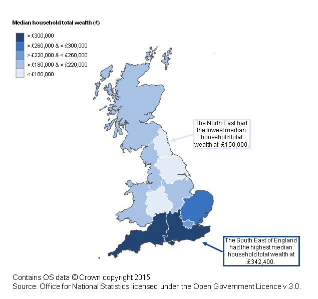
The median household total wealth for England rose by 3% to £228,200 between July 2010 to June 2012 and July 2012 to June 2014. In comparison, the median household total wealth for Scotland increased by 13% to £186,600 and the median household total wealth for Wales increased by 5% to £214,200. Looking at how the separate components of wealth have contributed to these changes (see separate chapters), Scotland saw an increase in all 4 wealth components, but most significantly in private pension wealth where the median increased by 60% (for those with such assets), compared with 24% for Wales and 19% for England. Conversely, Wales saw a fall in physical and financial wealth, but these were offset by the increases in property wealth and private pension wealth. In July 2012 to June 2014, the median household total wealth for Scotland is 13% lower than the corresponding value for Wales and 18% lower than the value for England.
Figure 2.12 presents the change in median household total wealth between July 2010 to June 2012 and July 2012 to June 2014 for all households by English region, Scotland and Wales. Six of the 9 regions of England saw an increase in median household total wealth, with households in London demonstrating the largest proportional rise – an increase of 14% in median household total wealth between July 2010 to June 2012 and July 2012 to June 2014. In terms of the wealth components, median household wealth in London increased for all components between July 2010 to June 2012 and July 2012 to June 2014 but was most considerable for private pension wealth and net property wealth (with rises of 16% and 9% respectively – for those with such assets).
In contrast, Yorkshire and The Humber saw a fall in median household total wealth of 8% between July 2010 to June 2012 and July 2012 to June 2014. Smaller falls were also seen in the West Midlands (2%) and East Midlands (1%). In terms of the wealth components, Yorkshire and The Humber saw a rise of 18% in median private pension wealth (for those with such assets) which was more than offset by falls in the median value of all other wealth components: median net financial wealth of households in Yorkshire and The Humber fell by 31%, median net property wealth fell by 8% and physical wealth by 5% between July 2010 to June 2012 and July 2012 to June 2014.
Great Britain, as a whole, saw a 4% increase in median household total wealth between July 2010 to June 2012 and July 2012 to June 2014.
Figure 2.12: Percentage change in household median total wealth, by region
Great Britain, July 2010 to June 2012 and July 2012 to June 2014
Source: Wealth and Assets Survey - Office for National Statistics
Download this chart Figure 2.12: Percentage change in household median total wealth, by region
Image .csv .xlsDistribution of household total wealth by household type
Figure 2.13 shows the distribution of total household wealth (including private pension wealth) by the composition of the household. It shows the 10 different categories for household type. It should be noted that some household types will have more adults than others. We would expect households with more than 1 adult to have higher levels of wealth than single person households because, in general, each additional adult makes a positive contribution to wealth accumulation.
Figure 2.13: Median household total wealth, by household type
Great Britain, July 2010 to June 2014
Source: Wealth and Assets Survey - Office for National Statistics
Download this chart Figure 2.13: Median household total wealth, by household type
Image .csv .xlsIn July 2012 to June 2014, the median value of household total wealth was the highest for couple households without children, where 1 person is over and the other under 60/651, at £678,000. The median value was next highest for couple households without children both over state pension age at 549,700. This median value of household total wealth for households in this latter group increased by some 26% between July 2010 to June 2012 and July 2012 to June 2014, compared with an increase of 14% for couple households without children, where 1 person is over and the other under 60/65.
The other household type with considerable median total household wealth in July 2012 to June 2014 was couple households with non-dependent children (£466,100), which had also seen a rise of some 15% between July 2010 to June 2012 and July 2012 to June 2014.
The type of household with the lowest median household total wealth across all 3 waves was ‘lone parent with dependent children’ with a median value of £26,800 in July 2012 to June 2014 (compared with £28,300 in July 2010 to June 2012).
The most common household type comprised couple households with dependent children, accounting for 19% of all households in the survey sample (23% of all individuals live in such households). These households had median total wealth of £190,600 in July 2012 to June 2014, a fall of 4% from July 2010 to June 2012.
Notes for household total wealth by main household characteristics
- 60/65 refers to women up to the age of 60 and men up to the age of 65.
7. Household total wealth by individual characteristics
This section looks at some main characteristics of individuals living in households with the various total wealth bands (including private pension wealth), where the lowest band of household total wealth includes negative total wealth. It is important to remember that analysis presents individual characteristics by the total wealth of the household that the individual lives within. In certain instances it is possible that this wealth is more likely attributed to other individuals living within that household.
Sex and marital status
Table 2.14 shows the distribution of individuals by sex and marital status, across the bands of household total wealth for the household in which they live. There is very little difference in the overall distribution of total wealth for men and women.
Married men and women are more likely to live in households of higher wealth, with 40% of married individuals living in households with a total wealth of £500,000 or more. Compared with single and cohabitating individuals, married individuals are on average older1. Knowing also that the earnings of older workers are higher than those of younger workers2 and that those older individuals will have had longer to accumulate wealth might go some way towards explaining these differences. Also, and compared with single individuals, those who were married might have accumulated more wealth if they were both working and in receipt of a higher joint income.
One might expect cohabiting individuals to be similar to married individuals, but over 60% of such individuals live in households with total wealth less than £200,000 (compared with less than a third of married individuals). This is most likely due to the fact that cohabiting individuals are generally much younger than married individuals1.
Widowed men and women are the next most likely to live in wealthier households – unsurprising as although such individuals often live in single adult households, they are also likely to be older and have inherited the wealth of their former spouse.
Single individuals do tend to live in households with less wealth, but the distribution is less skewed than for other marital status groups as some such individuals are young, but live with parents, whilst some are older and have accumulated more personal wealth.
Table 2.14: Individuals by sex and marital status, by household total wealth
| Great Britain, July 2012 to June 2014 | ||||||||
| % | ||||||||
| Less than £20,000 | £20,000 but < £85,000 | £85,000 but < £200,000 | £200,000 but < £300,000 | £300,000 but < £500,000 | £500,000 but < £1 million | £1 million or more | All Households | |
| Men | ||||||||
| Married | 5 | 11 | 15 | 11 | 17 | 23 | 17 | 100 |
| Cohabiting | 19 | 22 | 21 | 10 | 12 | 10 | 6 | 100 |
| Single | 19 | 19 | 17 | 10 | 13 | 14 | 8 | 100 |
| Widowed | 10 | 15 | 14 | 16 | 19 | 18 | 8 | 100 |
| Divorced | 21 | 16 | 17 | 12 | 13 | 14 | 6 | 100 |
| Separated | 23 | 20 | 23 | .. | 12 | 10 | .. | 100 |
| All men | 13 | 16 | 17 | 11 | 15 | 17 | 12 | 100 |
| Women | ||||||||
| Married | 5 | 11 | 15 | 11 | 17 | 23 | 17 | 100 |
| Cohabiting | 20 | 22 | 21 | 9 | 12 | 9 | 6 | 100 |
| Single | 22 | 19 | 18 | 9 | 12 | 12 | 8 | 100 |
| Widowed | 12 | 16 | 17 | 15 | 20 | 15 | 6 | 100 |
| Divorced | 22 | 19 | 19 | 11 | 15 | 10 | 3 | 100 |
| Separated | 29 | 25 | 18 | 8 | 10 | 7 | .. | 100 |
| All women | 15 | 16 | 17 | 11 | 15 | 16 | 11 | 100 |
| All Persons | 14 | 16 | 17 | 11 | 15 | 17 | 11 | 100 |
| Source: Office for National Statistics | ||||||||
| Notes: | ||||||||
| 1. Figures in italics are based on 30 or more unweighted cases but less than 50 - such data should be treated with some caution. | ||||||||
| 2. ".." - estimates that have been suppressed due to fewer than 30 unweighted cases. | ||||||||
Download this table Table 2.14: Individuals by sex and marital status, by household total wealth
.xls (27.6 kB)Age
Table 2.15 shows the distribution of individuals living in households with varying degrees of total wealth according to their age.
This table clearly shows the effect of wealth accumulation over the period of a lifetime. Individuals in the lowest age groups, that is, under the age of 35, were most likely to live in households with the lowest amounts of total wealth. In July 2012 to June 2014, 21% of 0 to 15 year olds, 16 to 24 year olds and 25 to 34 year olds were living in households with a total wealth of less than £20,000. Conversely, 6% of individuals who were aged 55 to 64 years and 7% of individuals aged 65 or older lived in households in the lowest total wealth band.
Now considering the highest total wealth band, 25% of all 55 to 64 year olds were living in households with total wealth of £1 million or more in July 2012 to June 2014. Individuals in this age group still find themselves in the wealth accumulation phase, and income, such as earnings from employment, enable opportunities to increase total wealth. Individuals aged 25 to 34 years old were the least likely to live in households in the top total wealth band (4%).
Table 2.15: Individuals by age, by household total wealth
| Great Britain, July 2012 to June 2014 | ||||||||
| % | ||||||||
| Less than £20,000 | £20,000 but < £85,000 | £85,000 but < £200,000 | £200,000 but < £300,000 | £300,000 but < £500,000 | £500,000 but < £1 million | £1 million or more | All Households | |
| Under 16 | 21 | 21 | 20 | 10 | 13 | 10 | 6 | 100 |
| 16-24 | 21 | 17 | 13 | 9 | 13 | 16 | 12 | 100 |
| 25-34 | 21 | 27 | 23 | 9 | 9 | 8 | 4 | 100 |
| 35-44 | 13 | 17 | 23 | 13 | 17 | 12 | 5 | 100 |
| 45-54 | 9 | 11 | 13 | 11 | 19 | 22 | 14 | 100 |
| 55-64 | 6 | 7 | 10 | 10 | 15 | 27 | 25 | 100 |
| 65+ | 7 | 10 | 13 | 12 | 20 | 24 | 16 | 100 |
| All persons | 14 | 16 | 17 | 11 | 15 | 17 | 11 | 100 |
| Source: Office for National Statistics | ||||||||
Download this table Table 2.15: Individuals by age, by household total wealth
.xls (26.6 kB)Education level
Table 2.16 shows the percentage of individuals living in households with varying degrees of household total wealth according to their education level.
Individuals who were educated to ‘degree level or above’ were the least likely to live in households in the bottom total wealth band of less than £20,000 (6%) and the most likely to live in households with total wealth of £1 million or more (23%), of all the education level groups in July 2012 to June 2014. The highest percentage of individuals living in households in the lowest band was amongst those with no formal educational qualifications (23%).
Table 2.16: Individuals by education level, by household total wealth
| Great Britain, July 2012 to June 2014 | ||||||||
| % | ||||||||
| Less than £20,000 | £20,000 but < £85,000 | £85,000 but < £200,000 | £200,000 but < £300,000 | £300,000 but < £500,000 | £500,000 but < £1 million | £1 million or more | All Households | |
| Degree level or above | 6 | 10 | 15 | 9 | 14 | 22 | 23 | 100 |
| Other qualifications | 12 | 16 | 16 | 11 | 17 | 18 | 10 | 100 |
| No qualifications | 23 | 18 | 18 | 12 | 15 | 11 | 4 | 100 |
| All persons1 | 12 | 15 | 16 | 11 | 16 | 18 | 13 | 100 |
| Source: Office for National Statistics | ||||||||
| Notes: | ||||||||
| 1. Includes only eligible adults that gave their education level. | ||||||||
Download this table Table 2.16: Individuals by education level, by household total wealth
.xls (26.6 kB)Economic activity
Table 2.17 considers the economic activity of individuals living in households across the different household total wealth bands.
In July 2012 to June 2014, of individuals who were economically inactive, 36% who gave their reasons for inactivity as ‘sick or disabled’ were from households in the lowest total wealth band of less than £20,000. Similarly, 36% of unemployed individuals were living in households within the lowest total wealth band. Retired or self-employed individuals were the least likely of all the economic activity groups to live in households within the lowest band of total wealth (7%).
As the values of the total wealth bands increase, the percentage of individuals in the different economic activity groups varies. In July 2012 to June 2014, the percentage of all individuals in the top total wealth category of ‘£1 million or more’ was 13%. Individuals who were retired were the most likely to live in households in the top wealth band of £1 million or more (18%). In comparison, 3% of economically inactive sick/disabled individuals were living in households in this top total wealth band.
Table 2.17: Individuals by economic activity, by household total wealth
| Great Britain, July 2012 to June 2014 | ||||||||
| % | ||||||||
| Less than £20,000 | £20,000 but < £85,000 | £85,000 but < £200,000 | £200,000 but < £300,000 | £300,000 but < £500,000 | £500,000 but < £1 million | £1 million or more | All Households | |
| Economically Active | ||||||||
| In Employment | 9 | 15 | 18 | 12 | 16 | 18 | 12 | 100 |
| Employee | 9 | 15 | 18 | 12 | 16 | 18 | 11 | 100 |
| Self Employed | 7 | 15 | 15 | 11 | 15 | 21 | 16 | 100 |
| Unemployed | 36 | 20 | 15 | 6 | 9 | 7 | 6 | 100 |
| Economically Inactive | ||||||||
| Student | 24 | 18 | 10 | 7 | 10 | 14 | 16 | 100 |
| Looking after family/home | 32 | 18 | 17 | 8 | 9 | 9 | 7 | 100 |
| Sick/Disabled1 | 36 | 24 | 16 | 7 | 8 | 6 | 3 | 100 |
| Retired | 7 | 9 | 12 | 11 | 19 | 23 | 18 | 100 |
| Other Inactive | 20 | 13 | 12 | 7 | 12 | 20 | 16 | 100 |
| All Persons | 12 | 15 | 16 | 11 | 16 | 18 | 13 | 100 |
| Source: Office for National Statistics | ||||||||
| Notes: | ||||||||
| 1. Combined figure for temporarily sick / injured and long term sick and disabled. | ||||||||
Download this table Table 2.17: Individuals by economic activity, by household total wealth
.xls (26.6 kB)Economic activity
Table 2.17 considers the economic activity of individuals living in households across the different household total wealth bands.
In July 2012 to June 2014, of individuals who were economically inactive, 36% who gave their reasons for inactivity as ‘sick or disabled’ were from households in the lowest total wealth band of less than £20,000. Similarly, 36% of unemployed individuals were living in households within the lowest total wealth band. Retired or self-employed individuals were the least likely of all the economic activity groups to live in households within the lowest band of total wealth (7%).
As the values of the total wealth bands increase, the percentage of individuals in the different economic activity groups varies. In July 2012 to June 2014, the percentage of all individuals in the top total wealth category of ‘£1 million or more’ was 13%. Individuals who were retired were the most likely to live in households in the top wealth band of £1 million or more (18%). In comparison, 3% of economically inactive sick/disabled individuals were living in households in this top total wealth band.
Table 2.18: Individuals by socio-economic classification, by household total wealth
| Great Britain, July 2012 to June 2014 | ||||||||
| % | ||||||||
| Less than £20,000 | £20,000 but < £85,000 | £85,000 but < £200,000 | £200,000 but < £300,000 | £300,000 but < £500,000 | £500,000 but < £1 million | £1 million or more | All Households | |
| Large employers and higher managerial | 2 | 7 | 14 | 10 | 17 | 25 | 26 | 100 |
| Higher professional | 4 | 11 | 16 | 10 | 18 | 23 | 18 | 100 |
| Lower managerial and professional | 8 | 13 | 17 | 12 | 18 | 21 | 11 | 100 |
| Intermediate occupations | 9 | 15 | 15 | 11 | 17 | 20 | 12 | 100 |
| Small employers and own account workers | 11 | 18 | 20 | 13 | 15 | 17 | 5 | 100 |
| Lower supervisory and technical | 18 | 20 | 18 | 12 | 14 | 13 | 5 | 100 |
| Semi-routine occupations | 23 | 22 | 19 | 12 | 12 | 9 | 3 | 100 |
| Routine occupations | 40 | 20 | 12 | 7 | 9 | 6 | 6 | 100 |
| Never worked/long term unemployed | 17 | 14 | 14 | 9 | 15 | 17 | 14 | 100 |
| All persons1 | 12 | 15 | 16 | 11 | 16 | 18 | 13 | 100 |
| Source: Office for National Statistics | ||||||||
| Notes: | ||||||||
| 1. Includes only adults who are 16 years old and above, not in full time education and gave sufficient information to determine socio-economic group. | ||||||||
| 2. Figures in italics are based on 30 or more unweighted cases but less than 50 - such data should be treated with some caution. | ||||||||
| 3. ".." - estimates that have been supressed due to fewer than 30 unweighted cases. | ||||||||
Download this table Table 2.18: Individuals by socio-economic classification, by household total wealth
.xls (26.6 kB)Notes for household total wealth by individual characteristics
See demographics in the Introductory Chapter.
Annual Survey of Hours and Earnings - Earnings by Age Group.