1. Main points
The gender pay gap for full-time workers is entirely in favour of men for all occupations; however, occupational crowding has an effect since those occupations with the smallest gender pay gap have almost equal employment shares between men and women.
When looking at age groups, the gap for full-time workers remains small at younger ages; however, from age 40 onwards the gap widens reaching its peak between ages 50 to 59.
Holding all other factors constant, for 2017 women’s pay growth in respect of age was lower than men’s pay growth and also stopped growing at a younger age.
Regarding job tenure, men who have worked for over 20 years in the same organisation earn 20.8% more compared with those men who worked for no longer than one year; for women, pay is 17.5% higher.
In terms of occupation, men working in the chief executives and senior officials occupation earn almost four times more than men in elementary occupations; in the case of women, this is almost 3.5 times more.
The Blinder-Oaxaca decomposition results show that 36.1% of the difference in men’s and women’s log hourly pay could be explained by differences in characteristics between men and women included in the model; of those, occupation has the largest effect since it explains 23.0% of the differences between men’s and women’s log hourly pay.
2. Introduction
The gender pay gap has always been a topic of interest, but in an attempt to increase awareness and improve pay equality, the UK government introduced compulsory reporting of the gender pay gap for organisations with 250 or more employees by April 20181. For the UK as a whole, the gap has reduced in the last 10 years but is still in favour of men2.
The gender pay gap is defined as the difference in median pay between men and women. The Office for National Statistics headline measure for the gender pay gap is calculated as the difference between median gross hourly earnings (excluding overtime) as a proportion of median gross hourly earnings (excluding overtime) for men. But crucially this measure does not take into account equal pay for equal work.
To summarise, this article will:
- present an overview of the Office for National Statistics headline measures for the gender pay gap, addressing the limitations of the estimation method used
- present analysis using regression modelling to explore some of the factors that affect men’s and women’s pay
- present experimental analysis that breaks down the gender pay gap by the factors that influence men’s and women’s pay
Notes for: Introduction
See Gender pay gap: overview for more information.
See The Annual Survey of Hours and Earnings: 2017 provisional and 2016 revised results, Section 7, Gender pay differences.
3. Things you need to know about this release
The analysis in this article uses data from the Annual Survey of Hours and Earnings (ASHE), which is the UK’s most comprehensive survey of individual employee pay. All estimates from the 2017 survey are provisional and relate to the reference date 26 April 2017. Data from the 2016 survey have been subject to small revisions since the provisional estimates were published on 26 October 2016.
Unless otherwise stated data referring to pay is excluding overtime. In section 4 data are reported in terms of median pay; in section 5 data refer to estimates of mean pay and in section 6 estimates of mean pay in log form. Only employees on adult rates, whose pay was not affected by sickness, are considered in the analysis. As a further point, employees without a valid work region or aged under 16 are not included. A full-time employee is defined as an employee who works more than 30 paid hours per week (or 25 or more for teaching professions). Note that no self-employed data is captured in ASHE.
Further information about ASHE can be found in quality and methodology, section 11 of this article, on our guidance and methodology page and in the Quality and Methodology Information (QMI) report.
Back to table of contents4. Headline measure
The Office for National Statistics headline measure for the gender pay gap uses Annual Survey of Hours and Earnings (ASHE) data and is calculated as the difference between median gross hourly earnings for men and women as a proportion of median gross hourly earnings for men. The analysis focuses on hourly earnings excluding overtime to control for the difference in the hours worked between men and women and the fact that men tend to work more overtime1.
In this section, analysis focuses on the headline gender pay gap measure, followed by the proportion of jobs by working pattern for men and women. Then, it focuses on occupation, showing the proportion of jobs and gender pay gap. Finally, the gender pay gap is reported by age groups and job tenure.
The headline measure for the gender pay gap
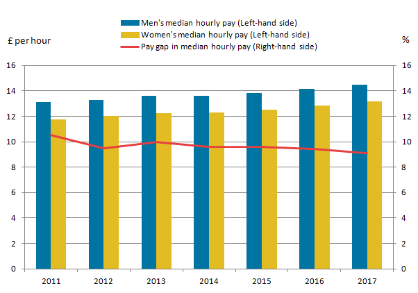
Figure 1 shows the median gross hourly earnings for men and women full-time employees. Between 2011 and 2017, men’s pay has grown by 10.4% from £13.12 to £14.48 per hour whilst women’s pay has grown by 12.0% from £11.75 to £13.16 per hour. In 2017, men on average were paid £1.32 more per hour than women, which, as a proportion of men’s pay, is a pay gap of 9.1%.
The pay gap has fallen from 10.5% in 2011 to 9.1% in 2017, but remains positive in value – meaning that on average men are paid more than women.
Figure 1: Median gross hourly earnings (excluding overtime) for full-time employees by sex, UK, 2011 to 2017
Source: Annual Survey of Hours and Earnings (ASHE) - Office for National Statistics
Notes:
- Employees on adult rates, pay unaffected by absence.
- Pay gap figures represent the difference between men's and women's hourly earnings as a percentage of men's earnings.
- Full-time is defined as employees working more than 30 paid hours per week (or 25 or more for the teaching professions).
- 2017 data are provisional.
Download this image Figure 1: Median gross hourly earnings (excluding overtime) for full-time employees by sex, UK, 2011 to 2017
.png (21.2 kB) .xls (27.6 kB)
The pay gap is useful in measuring pay equality due to its simple calculation; however, it does not measure the pay difference between men and women at the same pay grade, doing the same job, with the same working pattern. It also does not include any of the personal characteristics that may determine a person’s pay such as age.
Working patterns for men and women
Alternative measures of the pay gap allow for the control of the differences in the type of work that men and women do. One of the factors that affects pay for men and women is their working pattern. In 2017, the median hourly pay was higher for both men and women if they worked full-time compared with part-time workers. For men, median hourly pay for full-time work was 65.4% higher than for part-time work, and for women it was 42.8% higher2.
Figure 2 shows the proportions of men’s and women’s jobs that are full-time across different age groups. As can be seen, men are proportionally more likely to work full-time than women. At younger ages (16 to 21) men’s jobs are split almost equally between full-time (51.2%) and part-time (49.8%) but, between the ages of 30 to 39 (91.3%) and 40 to 49 (91.3%) more than 90% of men’s jobs are full-time. Women however, are less likely to work full-time, with only 61.1% and 57.6% of women’s jobs being full-time for ages 30 to 39 and 40 to 49 respectively.
Figure 2: Proportion of full-time men’s jobs and women’s jobs by working pattern and age group, UK, 2017
Source: Annual Survey of Hours and Earnings (ASHE) - Office for National Statistics
Notes:
- Employees on adult rates, pay unaffected by absence.
- Full-time is defined as employees working more than 30 paid hours per week (or 25 or more for the teaching professions).
- 2017 data are provisional.
Download this chart Figure 2: Proportion of full-time men’s jobs and women’s jobs by working pattern and age group, UK, 2017
Image .csv .xlsOccupation and the gender pay gap
Working pattern is not the only factor that can influence how much a job pays. Pay can also vary based on which occupation someone is employed in. When comparing hourly earnings for full-time employees men in the highest-paid occupation group (chief executives and senior officials) earn 5.3 times more than men in the lowest-paid occupation group (elementary occupations) whilst for women this figure is 4.5 times more.
When employment within an occupation is heavily skewed towards either men or women, it is likely to introduce occupational segregation – where some occupations become more attractive than others to either men or women.
Figure 3 shows the proportion of men and women full-time employees in each occupation group. Men have more than 60% share in six occupation groups whilst women have more than 60% share in only two groups, the remaining three occupation groups are roughly equal. Men have the highest employment share in skilled trade occupations with 92.0%. In contrast, women have the highest employment share in caring, leisure and other service occupations with 75.6%. Noticeably men have high proportion shares in the high-skill occupation groups (chief executives and senior officials, and managers and directors) and the low-skill occupation groups (elementary occupations, and process plant and machine operatives).
Figure 3: Proportion of men and women full-time employees by occupation, UK, 2017
Source: Annual Survey of Hours and Earnings (ASHE) - Office for National Statistics
Notes:
- Employees on adult rates, pay unaffected by absence.
- Full-time is defined as employees working more than 30 paid hours per week (or 25 or more for the teaching professions).
- 2017 data are provisional.
Download this chart Figure 3: Proportion of men and women full-time employees by occupation, UK, 2017
Image .csv .xlsIn 2017, men and women working full-time in the highest-paid occupation group (chief executives and senior officials) earned a median hourly pay of £48.53 and £36.54 respectively, men also had 72.8% of the full-time employment share in this occupation. Similarly, men had 70.2% of the full-time employment in the second-highest-paid occupation group (managers and directors) and had a median hourly pay of £23.69, which was £2.62 higher than the median hourly pay for women.
Figure 4 shows the gender pay gap for full-time and part-time workers in different occupations in 2017. For full-time workers, the pay gap is entirely in favour of men, the gap is largest in the skilled trade occupations group at 24.8% and smallest in sales and customer service occupations at 3.6%. Interestingly where the pay gap is largest (skilled trade occupations), men have the highest full-time employment share at 92.0% and where it is smallest (sales and customer service occupations), the full-time employment shares are almost equal with 50.1% men and 49.9% women. The respective hourly pay in that occupation is £9.62 for men and £9.27 for women.
Figure 4: Gender pay gap for median gross hourly earnings (excluding overtime) by occupation and working pattern, UK, 2017
Source: Annual Survey of Hours and Earnings (ASHE) - Office for National Statistics
Notes:
- Employees on adult rates, pay unaffected by absence.
- Pay gap figures represent the difference between men's and women's hourly earnings as a percentage of men's earnings.
- Full-time is defined as employees working more than 30 paid hours per week (or 25 or more for the teaching professions).
- 2017 data are provisional.
Download this chart Figure 4: Gender pay gap for median gross hourly earnings (excluding overtime) by occupation and working pattern, UK, 2017
Image .csv .xlsAge and the gender pay gap
One of the main characteristics that influences pay is someone’s age. This is because age approximates experience and in particular on-the-job training3 (this is a theme that is expanded on further in The impact of age in section 5). The analysis is therefore extended to look at the gender pay gap for people of similar age and working pattern.
Figure 5 shows the pay gap between men and women by age and working pattern. Across the younger age groups (16 to 21, 22 to 29 and 30 to 39), the gender pay gap is positive but relatively small for full-time workers (never greater than 2.4%). For part-time workers of the same age, the gap is negative. The widening of the pay gap in favour of women for those working part-time and aged 30 to 39 is likely to be influenced by the fact that the average age of first-time mothers is 28.8 years4 (continuing its upward trend) who may have a preference for part-time employment when rejoining the labour market (65.5% of mothers seek part-time work)5.
However, in older age groups (40 to 49, 50 to 59 and 60 and over) the pay gap is almost always positive for both full- and part-time workers. The increased gap for ages 40 to 49 and 50 to 59 may capture the differential impact of taking time out of the labour market. One possible reason for taking time out is having children; between April and June 2017, the employment rate for women with dependent children is 73.7% with 51.8% of the jobs being part-time whilst the employment rate for men with dependent children is 92.4% with 90.1% of these jobs being full-time6.
Figure 5: Gender pay gap for median gross hourly earnings (excluding overtime) by age group and working pattern, UK, 2017
Source: Annual Survey of Hours and Earnings (ASHE) - Office for National Statistics
Notes:
- Employees on adult rates, pay unaffected by absence.
- Pay gap figures represent the difference between men's and women's hourly earnings as a percentage of men's earnings.
- Full-time is defined as employees working more than 30 paid hours per week (or 25 or more for the teaching professions).
- 2017 data are provisional.
Download this chart Figure 5: Gender pay gap for median gross hourly earnings (excluding overtime) by age group and working pattern, UK, 2017
Image .csv .xlsJob tenure and the gender pay gap
Another characteristic that can approximate experience is the number of years a person has worked in a particular job. In 2017, the median hourly pay for men who worked full-time and had been in the same job for more than 20 years was £18.35, which was 59.6% higher than men who had been in their job for less than one year. Similarly, women who worked full-time and were in the same job for more than 20 years earned £16.16 per hour, 48.4% higher than women who had been in the same job for less than a year. Hence, somebody who has more years of service is likely to be paid more than someone who has just started. It is important to note here not all of the difference in pay can be attributed to the specific effect of job tenure.
Considering these differences, the analysis is refined to observe the gender pay gap for those with similar job tenures and working patterns.
Figure 6 displays the gender pay gap at differing levels of tenure for each working pattern. For full-time employees the gender pay gap is consistently positive in value indicating that for the levels of tenure compared, men are paid more than women. The pay gap is 5.3% for those who have been in their job for one year or less, and rises to 11.9% for those who have been in the same job for 20 or more years.
For part-time work the pay gap is negative for up to five years of employment in the same job. Women are paid 3.8% more than men when working in the same job for one year or less. After five years of employment in the same job, men begin to be paid more than women for part-time work with men earning 2.4% more. For those currently employed part-time who have been in the same job for more than 20 years the pay gap is 28.3%.
Figure 6: Gender pay gap for median gross hourly earnings (excluding overtime) by job tenure and working pattern, UK, 2017
Source: Annual Survey of Hours and Earnings (ASHE) - Office for National Statistics
Notes:
- Employees on adult rates, pay unaffected by absence.
- Pay gap figures represent the difference between men's and women's hourly earnings as a percentage of men's earnings.
- Full-time is defined as employees working more than 30 paid hours per week (or 25 or more for the teaching professions).
- 2017 data are provisional.
Download this chart Figure 6: Gender pay gap for median gross hourly earnings (excluding overtime) by job tenure and working pattern, UK, 2017
Image .csv .xlsNotes for: Headline measure
Data sourced from The Annual Survey of Hours and Earnings: 2017 provisional and 2016 revised results, Section 14. Hours paid.
Data sourced from The Annual Survey of Hours and Earnings: 2017 provisional and 2016 revised results, ASHE 1997 to 2017 selected estimates.
A relationship that was developed by Jacob Mincer in 1975: Mincer, J, 1975. Education, Experience and the Distribution of earnings and employment: An Overview. Education, Income, and Human Behaviour, n/a, pages 71 to 94.
Data sourced from Births by parents’ characteristics in England and Wales: 2016, Section 4. Average ages of mothers and fathers.
Data sourced from Families in the Labour Market 2017, Figure 16: Percentage of fathers and mothers (aged 16 to 64) who are looking for work.
Data sourced from Families in the Labour Market 2017, England, LFS and APS datasets: Table 3.
5. Modelling the factors that affect pay
Comparing the median pay differentials between men and women as a measure of the gender pay gap, as illustrated in section 4, only provides a partial picture. Men and women have different personal and job characteristics, which ultimately impact their respective pay. In this section, the analysis is developed using linear regression modelling to further illustrate the differences in pay between men and women.
Linear regression is a statistical technique that models a linear relationship between a dependent variable, and one or more explanatory variables (characteristics). In this model the log of hourly earnings is treated as the dependent variable and the explanatory variables are: age, job tenure, work pattern, occupation, region of work, business size and sector.
The advantage of modelling men’s and women’s pay using this technique is it enables the inclusion of multiple factors, holding these constant and observing the specific effect that each factor has. For example, the effect of each occupation group has on men’s and women’s pay can be analysed whilst holding the other factors constant. In this analysis the regression model that is estimated is applied separately to men and women and is estimated using ordinary least squares (OLS) regression. Note that due to the method of estimation used by OLS, data in this section are in mean and not median terms. For more information about the models, including the specification, see statistical notes 1 to 5 in section 10.
This section focuses on the regression results that cover the impact of age, job tenure and occupation.
The impact of age
In section 4, it was explained that age approximates experience, in this section this is expanded on. Economic theory suggests that pay is highly correlated with the accumulation of work experience, in other words, the more experience people have, the higher they are likely to be paid. The following analysis estimates the growth in mean hourly pay for men and women for 2017. It also assumes men and women have the same starting wage at age 16 and that all other modelled characteristics are held constant.
Figure 7 displays the growth in mean hourly pay for private sector full-time employees in 2017. Hourly wages grow with age for most of men’s and women’s working lives. For men, wages stop growing at 48, at which point they were 65.8% higher than the level at age 16, whilst for women, wages stopped growing at age 45 having increased by 50.4% compared with the level at age 16.
At the younger ages, men’s and women’s pay grow at similar rates, at the age of 24 men’s pay has grown by 2.9 percentage points more (since the level at age 16), but this divergence in growths continues and by the age of 48 men’s pay has grown 16.3 percentage points (since the level at age 16) more than women’s.
Figure 7: Index for the impact of age on the estimated mean hourly pay (excluding overtime) for full-time employees in the private sector, UK, age 16=100, 2017
Source: Annual Survey of Hours and Earnings (ASHE) - Office for National Statistics
Notes:
- Employees on adult rates, pay unaffected by absence.
- Full-time is defined as employees working more than 30 paid hours per week (or 25 or more for the teaching professions).
- Refer to reference tables for coefficients used to produce this analysis.
- 2017 data are provisional.
Download this chart Figure 7: Index for the impact of age on the estimated mean hourly pay (excluding overtime) for full-time employees in the private sector, UK, age 16=100, 2017
Image .csv .xlsFigure 8 displays the growth in mean hourly pay for public sector full-time employees in 2017. In the public sector, men’s and women’s pay stops growing at the same respective ages of 48 and 45 as they do in the private sector but the maximum level of growth is lower at 57.9% and 44.7% respectively.
Figure 8: Index for the impact of age on the estimated mean hourly pay (excluding overtime) for full-time employees in the public sector, UK, age 16=100, 2017
Source: Annual Survey of Hours and Earnings (ASHE) - Office for National Statistics
Notes:
- Employees on adult rates, pay unaffected by absence.
- Full-time is defined as employees working more than 30 paid hours per week (or 25 or more for the teaching professions).
- Refer to reference tables for coefficients used to produce this analysis.
- 2017 data are provisional.
Download this chart Figure 8: Index for the impact of age on the estimated mean hourly pay (excluding overtime) for full-time employees in the public sector, UK, age 16=100, 2017
Image .csv .xlsIn both the private and public sectors, wages grow faster for men and women at younger ages compared with growth at older ages. This analysis provides further evidence for the relationship between age (an approximate for experience) and pay1. The faster growth rates at younger ages reflect the higher accumulation of experience at younger ages. Looking at those aged 25 to 34 in England, employment rates for women are 19.8% lower for those with children compared with those without children2, for men the employment rates are 3.8% higher for those with children compared with those without children. As women with children are more likely than men with children to take time out of the labour market, a possible explanation for the divergence in pay is that men accumulate more experience than women over their working life.
The impact of tenure
Section 4 investigated the effect tenure had on men’s and women’s median hourly pay. In that analysis it was noted that men and women in full-time employment and working for more than 20 years in the same job earned 59.6% and 48.4% more respectively than men and women who had been in their job for less than one year.
In this section, the effect of tenure is shown on the mean hourly pay for men and women. Figure 9 illustrates the difference in mean hourly pay for men in 2017 as a result of different tenure groupings. All other factors are held constant and the effect is compared with those who have worked at the same organisation for no longer than one year.
As can be seen from Figure 9, men experience an increase in their mean hourly pay the longer they stay in their organisation. For men who have worked in an organisation for two to five years, the average effect is that they are paid 9.3% more; for those working in the same organisation for more than 20 years, they are paid 20.8% more than men who have been working for an organisation for less than a year.
Figure 9: The estimated difference in men’s mean hourly pay (excluding overtime) by job tenure group, UK, 2017
Source: Annual Survey of Hours and Earnings (ASHE) - Office for National Statistics
Notes:
- Employees on adult rates, pay unaffected by absence.
- Refer to reference tables for coefficients used to produce this analysis.
- 2017 data are provisional.
Download this chart Figure 9: The estimated difference in men’s mean hourly pay (excluding overtime) by job tenure group, UK, 2017
Image .csv .xlsFigure 10 on the other hand, illustrates the difference in mean hourly pay for women. Similarly to men, women also experience an increase in their mean hourly pay the longer they stay within an organisation. In comparison with women who have been in their job for less than one year, women in their job for more than 20 years experience on average pay 17.5% higher when all other factors are held constant.
Figure 10: The estimated difference in women’s mean hourly pay (excluding overtime) by job tenure group, UK, 2017
Source: Annual Survey of Hours and Earnings (ASHE) - Office for National Statistics
Notes:
- Employees on adult rates, pay unaffected by absence.
- Refer to reference tables for coefficients used to produce this analysis.
- 2017 data are provisional.
Download this chart Figure 10: The estimated difference in women’s mean hourly pay (excluding overtime) by job tenure group, UK, 2017
Image .csv .xlsThe impact of occupation
The analysis now focuses on the differences in mean hourly pay for each occupation in 2017 for men and women separately holding all other factors constant. For this analysis the changes in pay are in reference to the mean hourly pay earned by those working in elementary occupations.
Figure 11 shows the estimated difference in mean hourly pay for men in comparison with the reference group. The analysis shows that elementary occupations is the lowest-paying occupation group as all other occupations report a positive pay difference. In general, the higher-skill the occupation the larger the estimated pay difference, with the exception of other managers and proprietors. Men in the chief executives and senior officials occupation group achieve the highest estimated pay difference, earning almost four times (284.6%) more than men in elementary occupations when all other factors are held constant.
Figure 11: The estimated difference in men’s mean hourly pay (excluding overtime) by occupation, UK, 2017
Source: Annual Survey of Hours and Earnings (ASHE) - Office for National Statistics
Notes:
- Employees on adult rates, pay unaffected by absence.
- Refer to reference tables for coefficients used to produce this analysis.
- 2017 data are provisional.
Download this chart Figure 11: The estimated difference in men’s mean hourly pay (excluding overtime) by occupation, UK, 2017
Image .csv .xlsSimilarly, Figure 12 shows the estimated difference in the mean hourly pay for women in comparison with women in elementary occupations. Elementary occupations are also the lowest paying for women with all other occupations having a higher estimated pay. The estimated pay difference generally increases with skill although women in skilled trade occupations have an estimated pay difference of 10.7% compared with those in elementary occupations, which is lower than the 11.4% estimated in the caring, leisure and other service occupation group. Women in the highest skill group also achieve the highest pay difference, with women in the chief executives and senior officials occupation group earning almost 3.5 times (240.8%) more than those in elementary occupations.
Figure 12: The estimated difference in women’s mean hourly pay (excluding overtime) by occupation, UK, 2017
Source: Annual Survey of Hours and Earnings (ASHE) - Office for National Statistics
Notes:
- Employees on adult rates, pay unaffected by absence.
- Refer to reference tables for coefficients used to produce this analysis.
- 2017 data are provisional.
Download this chart Figure 12: The estimated difference in women’s mean hourly pay (excluding overtime) by occupation, UK, 2017
Image .csv .xlsNotes for: Modelling the factors that affect pay
Jacob Mincer in 1975: Mincer, J, 1975. Education, Experience and the Distribution of earnings and employment: An Overview. Education, Income, and Human Behaviour, n/a, pages 71 to 94.
Data sourced from Families in the Labour Market 2017, Figure 2 Employment rates of men and women with and without dependent children (aged 16 to 64) by age group, April to June 2017, England.
6. A breakdown of the gender pay gap
Section 5 showed that there are a number of factors that influence the pay of men and women differently. In this section, the pay gap is decomposed into an element that can be explained by the different characteristics held by men and women, and a remaining unexplained element. The Blinder-Oaxaca decomposition1 is used to perform this analysis.
This section builds on the analysis in section 5 using the regression models to observe the factors that influence the gender pay gap.
The decomposition estimates the explained element as the difference in pay caused by the different average levels of the characteristics held by men and women. This process assumes that men and women have exactly the same returns to those characteristics and that the men’s returns to characteristics are the equitable benchmark. For example, it assumes that women have the same returns to age as men and calculates whether women should earn more or less than men depending on whether they are on average older or younger. For more information on the decomposition method used please see statistical notes 6 through 9 in section 10.
The components in Figure 13 reflect each characteristic’s contribution to explaining the difference in log hourly earnings between men and women. A positive value reflects that men have favourable characteristics and therefore even if women had the same returns to those characteristics as men, and with all other factors held constant, there would still be a positive pay gap. The opposite is true for a negative value whereby women on average possess higher levels of a given characteristic than men, where that characteristic has a positive influence on pay.
Figure 13: The overall explained part and its components expressed as a percentage of the difference between log hourly earnings of men and women, UK, 2017
Source: Annual Survey of Hours and Earnings (ASHE) - Office for National Statistics
Notes:
- Employees on adult rates, pay unaffected by absence.
- Refer to reference tables for coefficients used to produce this analysis.
- 2017 data are provisional.
- The components are created by summing up the individual effect of each dummy variable.
Download this chart Figure 13: The overall explained part and its components expressed as a percentage of the difference between log hourly earnings of men and women, UK, 2017
Image .csv .xlsFigure 13 shows the results of the decomposition analysis. Of the difference between the log of men’s and women’s earnings, 36.1% can be explained by the difference in characteristics included in the model. Of the difference in log hourly earnings between men and women, 23.0% can be explained due to the different occupations that men and women work in. Whilst, 9.1% of the difference can be explained by the difference in working patterns, as was explained in section 4, men are more likely to work full-time, and full-time employees on average earn more. In other words, if women had the same returns to these characteristics as men and with all other factors held constant, women would still earn less on average than men because fewer women work in the highest-paying occupations and in full-time jobs.
In this analysis, it is assumed that the difference in log hourly earnings for men and women results in a pay differential in favour of men. This however, does not hold for age and business size characteristics because, if men’s and women’s returns to characteristics were the same and with all other factors held constant, the pay differential would be in favour of women.
Of the difference between the log of men’s and women’s earnings, 36.1% can be explained by the difference in characteristics included in the model. However, 63.9% of the gap cannot be explained. The analysis would benefit from information on family structures, education and career breaks; without these the unexplained element is over-stated. Factors such as the number of children, the age of children, whether parents have any caring responsibilities, the number of years spent in school and the highest level of qualification achieved are likely to improve the estimation of men’s and women’s pay structures and consequently decrease the unexplained element of the pay gap. As a result, the unexplained element should not be interpreted as a measure of discriminatory behaviour, though it is possible that this plays a part.
Notes for: A breakdown of the gender pay gap
- Blinder, A. S. (1973): Wage Discrimination: Reduced Form and Structural Estimates, in Journal of Human Resources 8(4), p. 436 to 455. Oaxaca, R. (1973). "Male-Female Wage Differentials in Urban Labor Markets". International Economic Review. 14 (3): 693 to 709.
7. Conclusions and next steps
Using the headline measure of gender pay gap, this article showed the gender pay gap for full-time workers is entirely in favour of men for all occupations. However, occupational crowding has an effect since those with the smallest gender pay gap also have almost equal employment shares between men and women. When looking at age groups, the gap for full-time workers remains small at younger ages. However, from 40 onwards the gap widens reaching its peak between ages 50 to 59 for full-time workers.
When we modelled the factors that influence pay, the results showed that both men’s and women’s pay grow for most of their lives. Overall, women’s pay grows less than men’s and also stops growing earlier than men’s pay. This applies to both the private and public sectors; however, the returns to pay are slightly lower in the latter.
Finally, according to the Blinder-Oaxaca decomposition results, 36.1% of the gender pay gap could be explained by differences in characteristics included in the model. From the characteristics considered, occupation has the largest effect since it explains 23.0% of the differences between men’s and women’s log hourly pay.
In conclusion, several factors affect men’s and women’s pay and thus the gender pay gap. From the ones analysed in this article, we found that occupation has the largest impact.
We consider our work has added to the existing research regarding the gender pay gap by showing experimental results using regression techniques. We would welcome any feedback you have regarding this article, particularly on any areas you would like to see developed further.
Back to table of contents9. References
Advisory, Conciliation and Arbitration Service and Government Equalities Office (2017) Gender pay gap reporting: overview.
Blinder, A. S. (1973) ‘Wage Discrimination: Reduced Form and Structural Estimates’. In Journal of Human Resources 8(4), pages 436 to 455.
Equality and Human Rights Commission (2017) The gender pay gap (PDF, 980KB). Research report 109.
Institute for Fiscal Studies (2016) The Gender Wage Gap (PDF, 429KB). IFS Briefing Note BN186.
Jann, B. (2008) ‘The Blinder-Oaxaca decomposition for linear regression models’. The Stata Journal, 8, Number 4, pages 453 to 479.
Mincer, J. (1975) Education, Experience and the Distribution of earnings and employment: An Overview (PDF, 518KB). Education, Income, and Human Behaviour, n/a, pages 71 to 94.
Oaxaca, R. (1973) ‘Male-Female Wage Differentials in Urban Labor Markets’. International Economic Review. 14(3), pages 693 to 709.
Office for National Statistics (2008) Modelling the gender pay gap in the UK: 1998 to 2006 (PDF, 285KB). Economic and Labour Market Review, Volume 2 Number 8 August 2008, pages 18 to 24.
Office for National Statistics (2014) Annual Survey of Hours and Earnings, Low Pay and Annual Survey of Hours and Earnings Pension Results Quality and Methodology Information.
Office for National Statistics (2016) Annual Survey of Hours and Earnings (ASHE) methodology and guidance.
Office for National Statistics (2016) Analysis of factors affecting earnings using Annual Survey of Hours and Earnings: 2016.
Office for National Statistics (2017) The Annual Survey of Hours and Earnings: 2017 provisional and 2016 revised results.
Office for National Statistics (2017) Families in the Labour Market 2017.
Office for National Statistics (2017) Births by parents’ characteristics in England and Wales: 2016.
Back to table of contents10. Statistical notes
Model specification (variable name in datasets):
Dependent variable:
- Log of hourly earnings excluding overtime (lnhexo)
Independent variables:
- Age (agel)
- Age2 (agesquare)
- Job tenure (tenure)
- Full- or part-time status (fulltime)
- Occupation classification, see quality and methodology (occu)
- Region of job location (region)
- Organisation size (bizsize)
- Sector (pubprivd)
Interaction terms:
- Sector*age & sector*age2
- Full-time*age & Full-time*age2
As a majority of the variables in the model are discrete, these have to be included as dummy variables. To avoid the issue of perfect multi-colinearity we have to omit one factor from each characteristic group that we can compare our analysis to, this omitted characteristic is known as the base category. The base categories selected for each variable are:
- Job tenure – Less than one year
- Full- or part-time status – Full-time
- Occupation – Elementary occupations
- Region – London
- Organisation size – Less than 10
- Sector – Private
The dependent variable is the log of hourly wages (excluding overtime). As the distribution of pay has a positive skew (earnings are distributed towards the lower end of distribution), taking the log of the variable helps normalise the distribution.
When accounting for the age of employees in the regression model, we have incorporated a variable for both age and age squared to help estimate the coefficients for the approximation for a known or unknown non-linear function of Χ, or in this case age.
As well as the suite of independent variables observed in the model, interaction terms are included. These are added to account for the fact that the proxy for work experience (Age and Age2) is different for people who work in different sectors and have different working patterns.
The presence of a significant interaction indicates that the effect of the first independent variable (x1) on the dependent variable (Y) is different at different values of a second independent variable (x2). It is tested by adding a term to the model in which the two independent variables are multiplied.
Y= β0 + β1*x1 + β2*x2 + β3*x1*x2
Adding an interaction term to a model drastically changes the interpretation of all of the coefficients. If there were no interaction term, β1 would be interpreted as the unique effect on the Y (in this case pay). But the interaction means that the effect of x1 on Y is different for different values of x2. So the unique effect of x1 is not limited to β1, but also depends on the values of β3 and x2.
The unique effect of x1 is represented by everything that is multiplied by x1 in the model:
- β1 + β3* x2
- β1 is now interpreted as the unique effect of x1 on Y only when x2= 0.
When interpreting the outputs of the model, care needs to be taken with the coefficients of variables. While the independent variables are in their original state, the dependent variable is in its log-transformed state, therefore, the coefficient (β) for the independent variables do not simply reflect the percentage change but (100*β)% for a one unit increase in the independent variable, with all other variable in the model held constant.
The Blinder-Oaxaca decomposition calculated in this article was performed using Stata and the downloadable ‘oaxaca’ command.
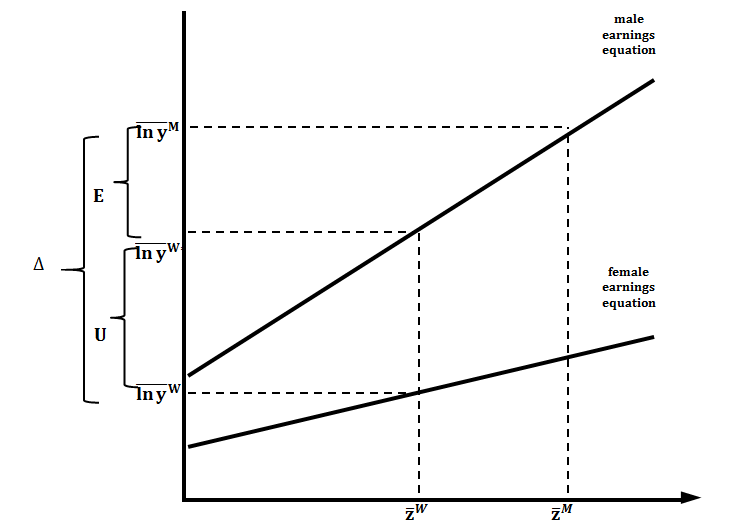
The decomposition uses the following linear regression property to estimate the mean log hourly earnings (excluding overtime) for men and women:
Where lnym is the estimated mean log hourly earnings (excluding overtime) for men and lnywis the estimated mean log hourly earnings (excluding overtime) for women. The means are estimated using the regression results reported in the dataset tables.
Through our analysis, the male earnings structure constitutes the benchmark and taken as non-discriminatory wage. Using this we estimate the counterfactual equation, which is the estimated mean hourly earnings (excluding overtime) for women if they had the same returns to their characteristics as men. The equation is therefore:
Running the decomposition analysis the difference between the mean hourly earnings (excluding overtime) between men and women can then be broken down into explained and unexplained parts:
Therefore the final decomposition equation is:
Figure 14 provides a simple visual representation of the decomposition analysis:
Figure 14: The Blinder-Oaxaca decomposition; a visual representation for a single explanatory variable
Download this image Figure 14: The Blinder-Oaxaca decomposition; a visual representation for a single explanatory variable
.png (15.8 kB)
11. Quality and methodology
This article presents analyses from the Annual Survey of Hours and Earnings (ASHE), the most detailed and comprehensive source of earnings information in the UK. ASHE is based on a 1% sample of employee jobs, drawn from HM Revenue and Customs Pay as You Earn (PAYE) records. It does not cover the self-employed nor does it cover employees not paid during the reference period.
The figures in ASHE relate to the reference date of 26 April 2017 and thus capture the early effects of the changes to the National Living Wage (£7.50) for employees aged 25 and over on 1 April 2017, as well as the changes to the National Minimum Wage of other age groups (£7.05 for those aged 21 to 24, £5.60 for those aged 18 to 20, £4.05 for those aged under 18 and £3.50 for apprentices aged under 19 or in the first year of their apprenticeship), which also occurred on the same date.
Quality and Methodology Information
The Annual Survey of Hours and Earnings Quality and Methodology Information report contains important information on:
- the strengths and limitations of the data
- the quality of the output: including the accuracy of the data and how it compares with related data
- uses and users
- how the output was created
Relevance
The earnings information in ASHE relates to gross pay before tax, National Insurance or other deductions and excludes payments in kind. With the exception of annual earnings, the results are restricted to earnings relating to the survey pay period and so exclude payments of arrears from another period made during the survey period; any payments due as a result of a pay settlement but not yet paid at the time of the survey will also be excluded.
Most of the published ASHE analyses (that is, excluding annual earnings) relate to employees on adult rates whose earnings for the survey pay period were not affected by absence. They do not include the earnings of those who did not work a full week and whose earnings were reduced for other reasons, such as sickness. Also, they do not include the earnings of employees not on adult rates of pay, most of whom will be young people. More information on the earnings of young people and part-time employees is available in the main survey results. Full-time employees are defined as those who work more than 30 paid hours per week or those in teaching professions working 25 paid hours or more per week.
Sampling error
ASHE aims to provide high quality statistics on the structure of earnings for various industrial, geographical, occupational and age-related breakdowns. However, the quality of these statistics varies depending on various sources of error.
Sampling error results from differences between a target population and a sample of that population. Sampling error varies partly according to the sample size for any particular breakdown or “domain”.
Non-sampling error
ASHE statistics are also subject to non-sampling errors. For example, there are known differences between the coverage of the ASHE sample and the target population (that is, all employee jobs). Jobs that are not registered on PAYE schemes are not surveyed. These jobs are known to be different to the PAYE population in the sense that they typically have low levels of pay. Consequently, ASHE estimates of average pay are likely to be biased upwards with respect to the actual average pay of the employee population. Non-response bias may also affect ASHE estimates. This may happen if the jobs for which respondents do not provide information are different to the jobs for which respondents do provide information. For ASHE, this is likely to be a downward bias on earnings estimates since non-response is known to affect high-paying occupations more than low-paying occupations.
Further information about the quality of ASHE (PDF, 57KB), including a more detailed discussion of coverage and non-response errors, is available on our archive website.
Re-weighting of the Labour Force Survey
Returned data from ASHE are weighted to UK population totals from the Labour Force Survey (LFS). The LFS itself has recently been reweighted, using revised UK and subnational population estimates consistent with the 2011 Census and updated population projections. The impact of this on the ASHE results is negligible. Further information on the LFS reweighting can be found on our LFS user guidance pages.
Classification of SOC 2010
The Standard Occupational Classification 2010: SOC 2010 separates the labour market into nine major groups, based on criteria such as the qualifications, skills and experience associated with each job.
This article uses those nine major groups but breaks down the first major grouping, managers, directors and senior officials, into three groups. These groups are: chief executives and senior officials, managers and directors, and other managers and proprietors. Table 1 describes the features of each grouping.
Table 1: SOC2010 classification groupings and share of employee’s by grouping, UK, 2017
| Grouping | SOC2010 Code | Proportion of men, ASHE 2017 | Proportion of women, ASHE 2017 | |||
|---|---|---|---|---|---|---|
| Chief Executives and Senior Officials | 1110-1119 | 0.5 | 0.2 | |||
| Managers and Directors | 1120-1199 | 10.5 | 5.2 | |||
| Other Managers & Proprietors | 1200-1299 | 1.7 | 1.6 | |||
| Professional occus | 2100-2999 | 20.6 | 22.5 | |||
| Associate Professional and Technical occus | 3100-3999 | 16.5 | 12.8 | |||
| Administrative and Secretarial occus | 4100-4999 | 5.8 | 17.8 | |||
| Skilled Trades occus | 5100-5999 | 12.9 | 1.7 | |||
| Caring, Leisure and Other Service occus | 6100-6999 | 3.5 | 15.6 | |||
| Sales and Customer Service occus | 7100-7999 | 6.1 | 10.1 | |||
| Process, Plant and Machine Operatives | 8100-8999 | 10.2 | 1.5 | |||
| Elementary Occupations | 9100-9999 | 11.4 | 11.1 | |||
| Source: Annual Survey for Hours and Earnings | ||||||
Download this table Table 1: SOC2010 classification groupings and share of employee’s by grouping, UK, 2017
.xls (28.7 kB)In March 2012, the 2011 ASHE estimates were published on a Standard Occupational Classification (SOC) 2010 basis (they had previously been published on a SOC 2000 basis). Since the SOC forms part of the methodology by which ASHE data are weighted to produce estimates for the UK, this release marked the start of a new time series and therefore care should be taken when making comparisons with earlier years.
Similarly, methodological changes in 2004 and 2006 also resulted in discontinuities in the ASHE time series. On 28 February 2014 we published a methodological note explaining the impact of the change in Standard Occupational Classification on the estimates of public and private sector pay.
Back to table of contents