Income estimates for small areas, England and Wales: financial year ending 2014

In 2013/14 (the financial year ending 2014), average total (gross) household income in small areas within England and Wales ranged from £340 per week to £1,710, with around half of small areas falling in the £500 to £750 per week income band.

Average weekly household income in 2013/14 was highest in London and its surrounding areas.

Areas of lowest average household incomes were more widely spread across England and Wales than were the areas of highest incomes.

This bulletin presents the official estimates of household income. They are accompanied by Administrative Data Census Research Outputs on individual income for local authority districts in England and Wales, which are not official statistics, but have been produced from administrative data on income and benefits.

The small area model-based income estimates are the official estimates of weekly household income at the middle layer super output area (MSOA) level in England and Wales for 2013/14 (the financial year ending 2014)¹. They are designated National Statistics which are calculated using a model-based method to produce 4 estimates of income. The estimates are produced using a combination of survey data from the Family Resources Survey and previously published data from the 2011 Census and a number of administrative data sources. The 4 different measures of income are:

1. total (gross) weekly household income

2. net weekly household income

3. net weekly household income (equivalised²) before housing costs

4. net weekly household income (equivalised²) after housing costs

The first 2 measures provide an indication of both average (mean) overall household income and average household income after taking into account tax payments and housing costs. The last 2 measures provide equivalised estimates of household income which take into account the composition of households. This enables meaningful comparisons between households with different numbers of occupants.

The estimates described in this statistical bulletin are accompanied by Administrative Data Research Outputs on income, which have been produced from administrative data on income and benefits. The Research Outputs are available for local authority districts in England and Wales for the financial year ending March 2014. These Research Outputs are NOT official statistics. They should not be interpreted as an indicator of poverty or living standards. Rather they are published as outputs from research into a different methodology to that currently used in the production of income statistics. Income recorded via self-assessment (which includes income received from self-employment, property rental and investments) and some benefits are not included in the Research Outputs.

For the small area model-based income estimates in this bulletin, you might find it helpful to read our user guide to the small area income estimates, which accompanied the release of the previous estimates, but also applies to this release. There is also more detailed information about the method and data sources used to produce these estimates, available in the technical report released alongside the data and this statistical bulletin.

The small area income estimates are particularly useful for local authority planning. They are used to support effective service provision, targeting of resources and the allocation of grants and funding. They are also used by a range of government policymakers, businesses and academic organisations for various purposes including:

• assessing the relationship between local economies, industry sectors and income
• combining income data with indicators from related topics such as skills, employment, migration and housing
• strategic planning of site locations and forecasting by businesses

This statistical bulletin presents the results of the 2013/14 small area income estimates for each of the 4 types of income at the middle layer super output area (MSOA) level. The geographic distribution of each type of average household income is described along with analysis of the overall distribution for different income bands.

These income estimates can be used to provide an indication of changes in household income over time, providing that the 95% confidence intervals, presented with the estimates, are considered. For example, if there is no overlap in the confidence intervals of an MSOA’s estimate of income at 2 points in time, then this provides an indication that mean weekly household income has changed in this area. For more information about identifying changes in estimated income over time, see the technical report [insert link to technical report once known] which accompanies these estimates.

Notes for: Things you need to know about this release

1. Throughout this release, 2013/14 refers to the financial year ending 2014; April 2013 to March 2014 and likewise for earlier years.

2. See section 4 for more information about equivalisation.

Total weekly household income is the sum of the gross income of every member of the household plus any income from benefits such as Working Families Tax Credit. This measure is particularly useful for understanding the average level of income from earnings and investments, as it is not affected by payments of tax or other deductions. It is calculated as the sum of income from:

• wages and salaries (gross)
• self-employment
• investments
• tax credits
• State Pension and Income Support or Pension Credit
• other pensions
• other benefits
• disability benefits
• other sources of income

London and the areas surrounding it contained most of the areas in which average (mean) total weekly household income was highest. In 2013/14 (the financial year ending 2014), 40 of the top 50 middle layer super output areas (MSOAs) for average total weekly household income were in London and the others were relatively close to London, in the neighbouring East of England and South East regions. Areas with relatively high income can reflect the fact that a small number of households in those areas can have particularly high income relative to other households in the same area.

Looking at the top 50 areas for average weekly income is useful in giving an indication of the highest level of average income because this approach helps to negate uncertainty around the estimates. Figure 1 shows that in 2013/14, clusters of MSOAs that had relatively high average household income outside of London and its surrounding areas were less common than within London.

The map shows that MSOAs in the South East appear to have particularly high household income relative to MSOAs in bordering regions. This is partly a result of the method used to estimate income, whereby all MSOAs within a region have been adjusted to align them more closely with household income in the region as a whole. Therefore, care should be taken when comparing the income of MSOAs across regions, particularly for MSOAs that are close to regional borders. The confidence intervals presented with these estimates provide an indication of the uncertainty around each MSOA’s estimate of household income. For more detailed information about the method used to produce these estimates, see the technical report.

The areas that had the lowest average total weekly household income were generally more spread out geographically than areas in which household income was higher. For example, cities and larger towns across England and Wales tended to have some areas of relatively low income within them, but not all had areas of particularly high income. This is partly explained by the fact that income in many of London’s MSOAs was notably higher than income in other cities’ MSOAs. However, parts of England and Wales had groupings of areas that had relatively low income in 2013/14. These include Birmingham, Liverpool, County Durham and Nottingham.

Figure 1: Model-based mean total weekly household income by middle layer super output area

England and Wales, 2013/14

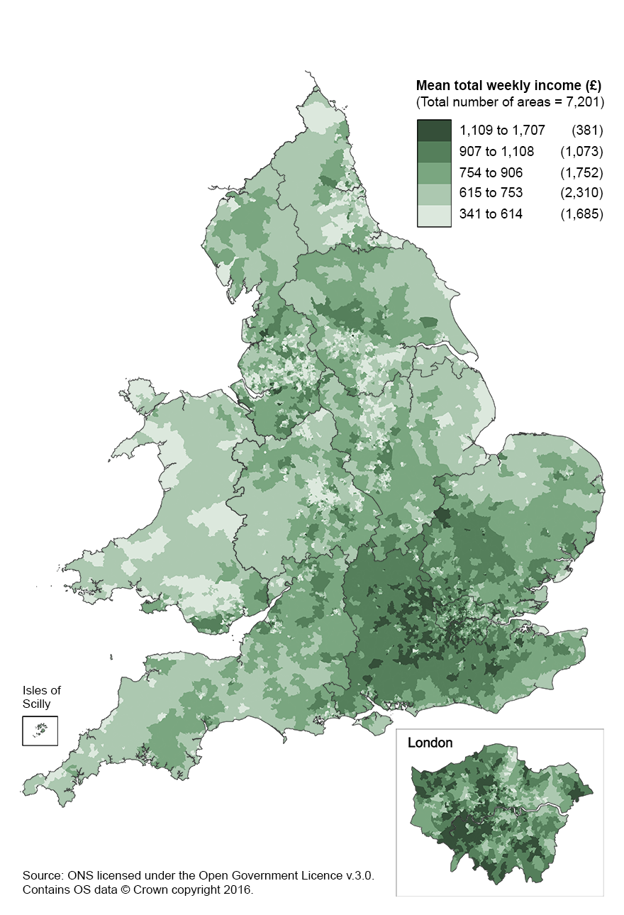
Source: Office for National Statistics licensed under the Open Government Licence v.3.0. Contains Ordnance Survey data © Crown copyright and database right 2016

Download this image Figure 1: Model-based mean total weekly household income by middle layer super output area

.png (646.2 kB)

Figure 2 shows that the £615 to £751 income band was the band that had the largest number of MSOAs in 2013/14. It also shows that some areas in the higher income bands had particularly high levels of average household income, whereas a larger number of areas fall within the lower income brackets. This is typical of the distribution of household income.

MSOA level estimates allow the exploration of differences in mean household income within local authority districts (LADs) to better understand income at the local level, whilst taking account of the uncertainty around the estimates described by the 95% confidence intervals.

The distribution of weekly household income varies across LADs, even for LADs within the same region, particularly within London and the South East of England. There are LADs that did not contain any MSOAs in the same band as another LAD in the same region. For example, Figure 3 shows the number of MSOAs within each income band for Barking and Dagenham, and for Richmond upon Thames. Both LADs are in London but had very different MSOA distributions in 2013/14. In Barking and Dagenham the income band with the most MSOAs in was the £570 to £674 per week band. For Richmond upon Thames the income band with the most MSOAs in was the £1,200 to £1,304 per week band.

Despite Richmond upon Thames having a wider range of weekly household income than Barking and Dagenham, there were no income bands that contained MSOAs from both LADs. This shows that the distribution household income for small areas within London boroughs can differ greatly.

The estimates for MSOAs within an LAD can be described as significantly different if the confidence intervals for the estimates do not overlap. This bulletin provides examples of some LADs in which the MSOA with the highest income was significantly different to all other MSOAs in that LAD. This provides an illustration of how these estimates can be used to identify areas of particularly high household income within an LAD.

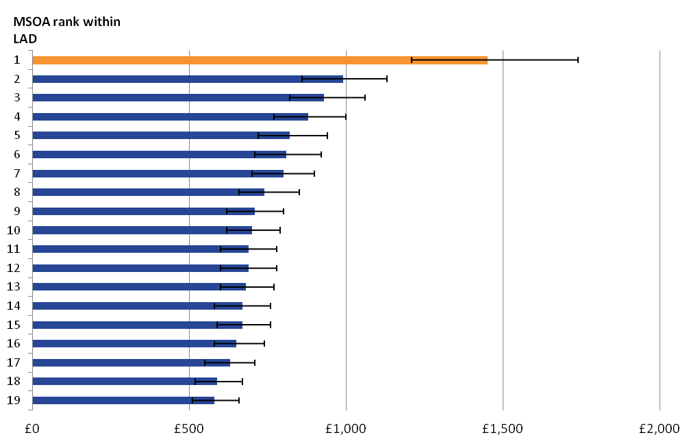
Figure 4 shows the mean total weekly household income (with 95% confidence intervals) for the 19 MSOAs in the Thurrock LAD. This LAD had the largest proportion of MSOAs with estimates that were significantly lower than the MSOA that had the highest mean total income in the LAD. All of the other 18 MSOAs had significantly lower mean total income.

Figure 4: Mean total weekly household incomefor middle layer super output areas within local authority districts

Thurrock, 2013/14

Source: Office for National Statistics

Notes:

1. Ranked by highest mean total weekly household income.

Download this image Figure 4: Mean total weekly household incomefor middle layer super output areas within local authority districts

.png (12.3 kB) .xls (28.7 kB)

Other LADs containing a similarly high proportion of MSOAs with lower total income compared with the highest ranked MSOA were Leicester (35 out of 37) and Reading (17 out of 18). However, not all LADs show this pattern. South Cambridgeshire contains 20 MSOAs in which none had significantly different mean total weekly household income than the highest ranked MSOA.

Conversely, the LAD with the largest proportion of MSOAs with significantly higher total income than the lowest ranked MSOA was Stockport (39 out of 42).

Net weekly household income (unequivalised¹) is the sum of the net income of every member of the household. It is useful when assessing the average levels of income having taken account of common deductions from salary. For example, the average net weekly income might be significantly higher in one area than in another, despite these areas having similar level of average total weekly income. This would indicate that factors such as Council Tax payments account for some of the difference in income, rather than the average amount of earnings alone. The net weekly measure of average income does not take account of different areas having different household compositions and so is also useful in assessing the extent to which the number of people and their characteristics influence average household income. This is explained further in later sections of the bulletin.

Net weekly household income is calculated using the same components as total income but income is net of:

• Income Tax payments
• National Insurance contributions
• domestic rates or Council Tax
• contributions to occupational pension schemes
• all maintenance and child support payments, which are deducted from the income of the person making the payments
• parental contribution to students living away from home

For some middle layer super output areas (MSOAs), the modelled estimate of net weekly household income was greater than the modelled estimate of total income. This is the result of the method used to produce the estimates, which use a separate statistical model for each type of income. In reality, total household income is always higher than net household income and so care should be taken when comparing estimates of total income with estimates of net income. The confidence intervals presented with these estimates provide an indication of the uncertainty around each MSOA’s estimate of the different types of household income. For more detailed information about the method used to produce these estimates, see the technical report.

Figure 5 shows the estimates of equivalised net weekly income. Middle layer super output areas (MSOAs) where net weekly income was highest in 2013/14 (the financial year ending 2014) are in and around the South East and London.

As for total income, the map for net household income shows that MSOAs in the South East appear to have particularly high household income relative to MSOAs in bordering regions. This is partly a result of the method used to estimate income, whereby all MSOAs within a region have been adjusted to align them more closely with household income in the region as a whole. Therefore, care should be taken when comparing the income of MSOAs across regions, particularly for MSOAs that are close to regional borders.

Figure 5: Model-based mean net weekly household income (unequivalised) by middle layer super output area

England and Wales, 2013/14

Source: Office for National Statistics licensed under the Open Government Licence v.3.0. Contains Ordnance Survey data © Crown copyright and database right 2016

Download this image Figure 5: Model-based mean net weekly household income (unequivalised) by middle layer super output area

.png (647.4 kB)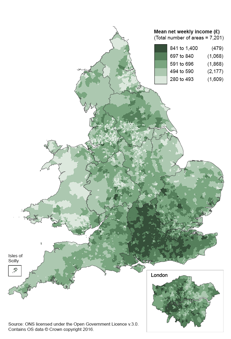

Figure 6 shows the distribution of MSOAs for mean net weekly household income. Although the ranges differ from mean total household income, the distribution is quite similar. It is not as positively skewed, although there are some areas that fall within relatively high income groups. This could be due to the highest earning households paying proportionately more in mandatory charges such as Income Tax.

Figure 7 shows the mean net weekly household income (with 95% confidence intervals) for the 37 MSOAs in the Leicester local authority district (LAD). This LAD had the largest proportion of MSOAs with estimates that were significantly lower than the MSOA that had the highest mean net income in the LAD. All of the other 36 MSOAs had significantly lower net income.

Figure 7: Mean net weekly household income for middle layer super output areas within local authority districts

Leicester, 2013/14

Source: Office for National Statistics

Notes:

1. Ranked by highest mean net weekly household income.

Download this image Figure 7: Mean net weekly household income for middle layer super output areas within local authority districts

.png (14.1 kB) .xls (29.2 kB)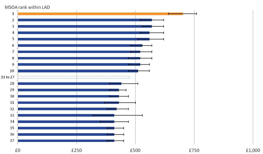

Other LADs containing a similarly high proportion of MSOAs with lower net income compared with the highest ranked MSOA were South Tyneside (22 out of 23) and Wakefield (43 out of 45). However, not all LADs show this pattern. South Lakeland LAD contains 14 MSOAs in which none had significantly different mean net weekly household income than the highest ranked MSOA.

Conversely, the LAD with the largest proportion of MSOAs with significantly higher net income than the lowest ranked MSOA was Salford (29 out of 30).

Net weekly household income before housing costs (equivalised) is composed of the same elements as net weekly household income but is subject to an equivalisation scale. Applying an equivalisation scale adjusts the household income values to take account of the number and composition of people in the household. Therefore, it represents the income level of every individual in the household.

Equivalisation is needed in order to make sensible income comparisons between households. For example, one household may have 2 adults and 2 children and have a total weekly household income of £300. If this is compared with a household containing just 1 adult who has a total weekly household income of £270, then although the first household has the higher total weekly income it is the second that has the higher standard of living (assuming equal living and housing expenses).

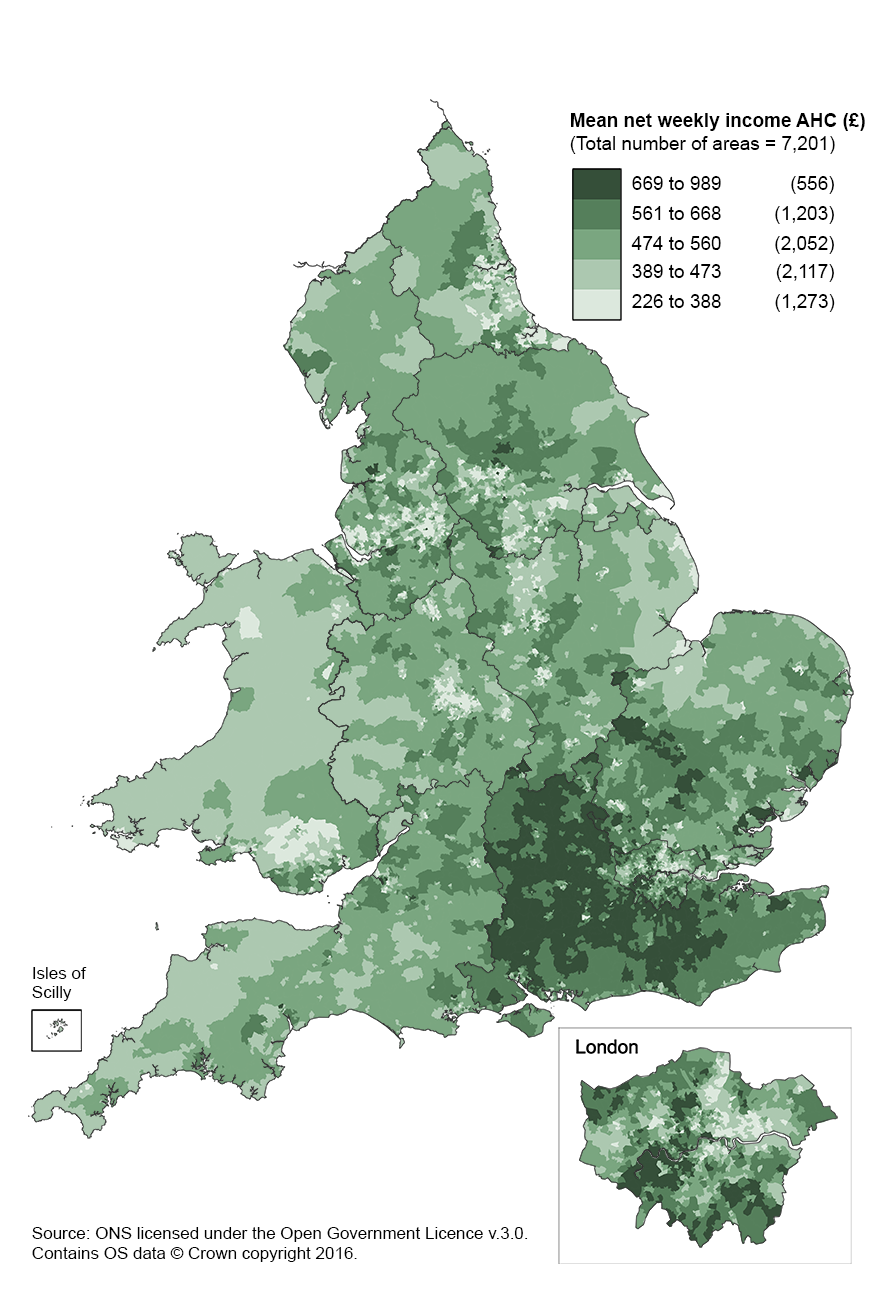
Geographically, mean net weekly household income (equivalised) before housing costs (BHC) broadly follows the same trends as mean net weekly household income in that middle layer super output areas (MSOAs) with the highest weekly income were predominantly in and around London and the South East. Figure 8 shows that the estimates of equivalised net weekly income themselves are also similar to the estimates of net weekly income, with more than 95% of areas for the equivalised estimates falling within plus or minus 17% of the unequivalised estimates.

Similar to the maps for unequivalised income, the map for equivalised BHC income shows that MSOAs in the South East appear to have particularly high household income relative to MSOAs in bordering regions. This is partly a result of the method used to estimate income, whereby all MSOAs within a region have been adjusted to align them more closely with household income in the region as a whole. Therefore, care should be taken when comparing the income of MSOAs across regions, particularly for MSOAs that are close to regional borders. The confidence intervals presented with these estimates provide an indication of the uncertainty around each MSOA’s estimate of household income. For more detailed information about the method used to produce these estimates, see the technical report.

Figure 8: Model-based mean net weekly household income (equivalised) before housing costs by middle layer super output area

England and Wales, 2013/14

Source: Office for National Statistics licensed under the Open Government Licence v.3.0. Contains Ordnance Survey data © Crown copyright and database right 2016

Download this image Figure 8: Model-based mean net weekly household income (equivalised) before housing costs by middle layer super output area

.png (639.7 kB)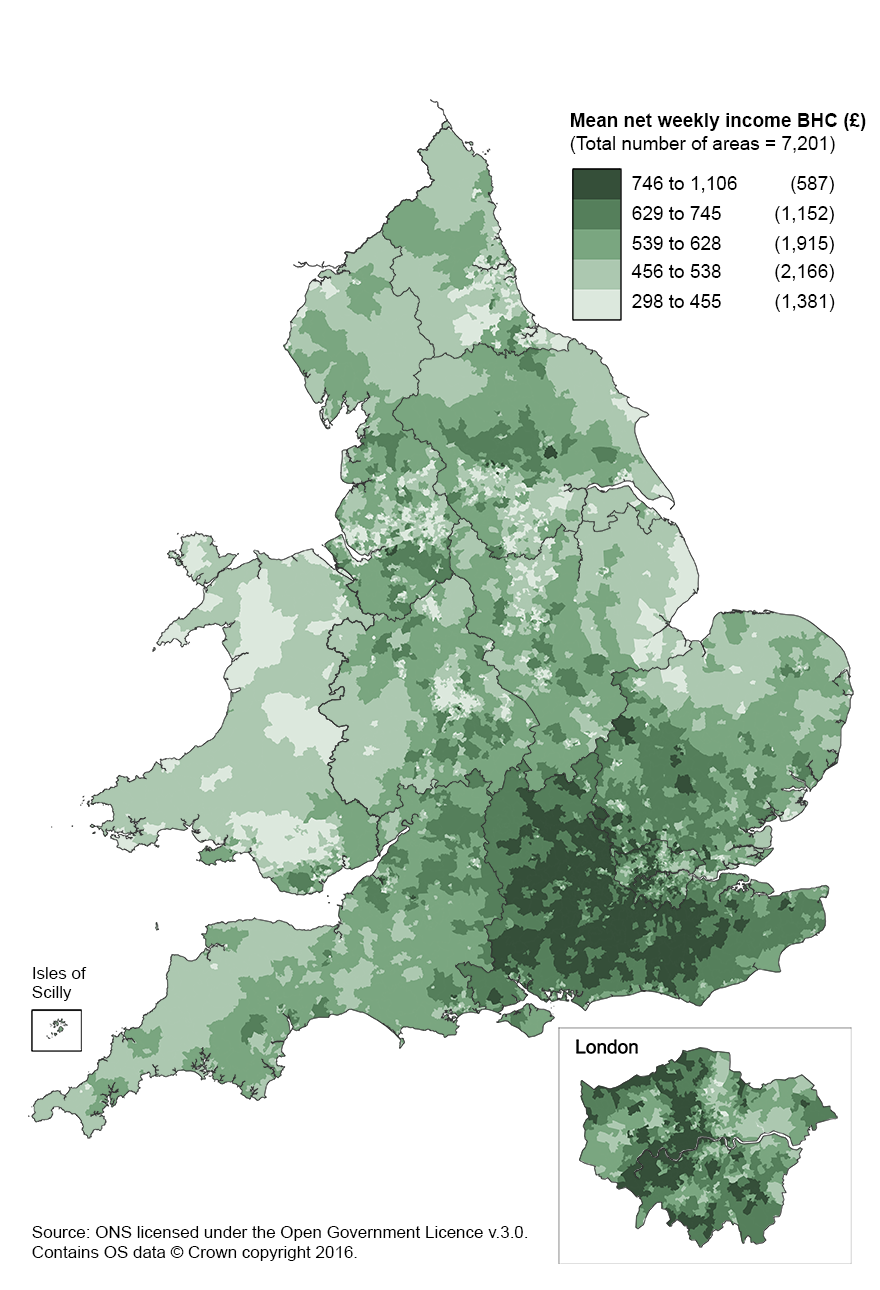

Although the ranges differ from mean unequivalised net household income, Figure 9 shows that the distribution of MSOAs for average net weekly household income (equivalised) before housing costs broadly follows the same distribution.

Figure 10 shows the mean net weekly household income (equivalised) before housing costs (with 95% confidence intervals) for the 70 MSOAs in Sheffield local authority district (LAD). This LAD had the largest proportion of MSOAs with estimates that were significantly lower than the MSOA that had the highest mean net income before housing costs in the LAD. All of the other 69 MSOAs had significantly lower total income.

Figure 10: Mean net weekly household income (equivalised) before housing costs for middle layer super output areas within local authority districts

Sheffield, 2013/14

Source: Office for National Statistics

Notes:

1. Ranked by highest mean net weekly household income (equivalised) before housing costs.

Download this image Figure 10: Mean net weekly household income (equivalised) before housing costs for middle layer super output areas within local authority districts

.png (14.3 kB) .xls (29.2 kB)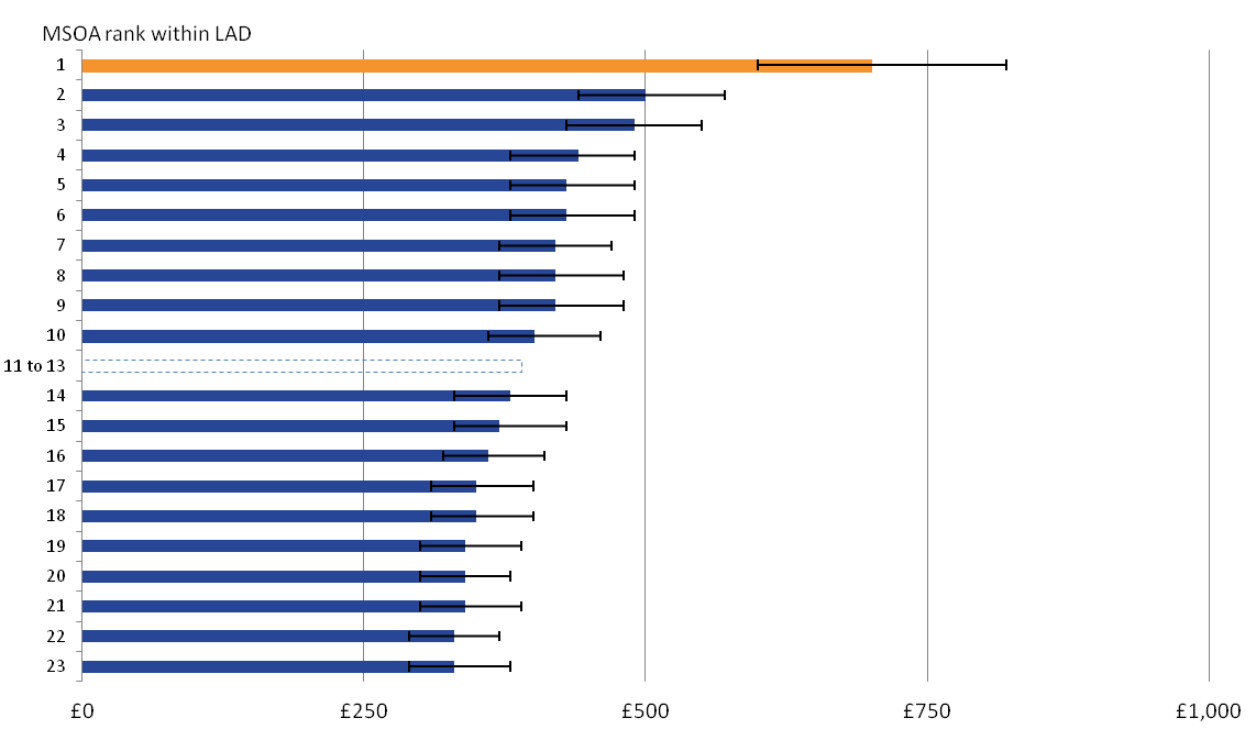

Birmingham had a similarly high proportion, with 128 out of 132 MSOAs with significantly lower net BHC income compared with the highest ranked MSOA. However, not all LADs show this pattern. For example, West Oxfordshire contains 15 MSOAs in which none had significantly different mean net (BHC) income than the highest ranked MSOA.

Conversely, the LAD with the largest proportion of MSOAs with significantly higher net BHC income than the lowest ranked MSOA was Huntingdonshire (21 out of 22).

Net weekly household income after housing costs (equivalised) is composed of the same elements of net weekly household income but is subject to the following deductions prior to an equivalisation scale being applied:

• rent (gross of housing benefit)
• water rates, community water charges and council water charges
• mortgage interest payments (net of any tax relief)
• structural insurance premiums (for owner occupiers)
• ground rent and service charges

Net weekly household income (equivalised) after housing costs (AHC) is particularly useful for assessing the impact of the costs of housing for a given area and for providing an indicator of disposable income before the cost of living. For example, if one area has significantly higher average household income before housing costs but similar average income after housing costs, we can deduce that the costs of housing are greater in that area.

However, for some middle layer super output areas (MSOAs), the modelled estimate of net weekly household income (equivalised) after housing costs was greater than the modelled estimate of income before housing costs. This is the result of the method used to produce the estimates, which use a separate statistical model for each type of income. In reality, income before housing costs is always higher than income after housing costs and so care should be taken when comparing these estimates. The confidence intervals presented with these estimates provide an indication of the uncertainty around each MSOA’s estimate of household income for the different types of income. For more detailed information about the method used to produce these estimates, see the technical report.

Figure 11 shows that average income on this measure is broadly consistent geographically with the other measures of net income. Similar to the maps for the other measures of income, the map for equivalised AHC income shows that MSOAs in the South East appear to have particularly high household income relative to MSOAs in bordering regions. This is partly a result of the method used to estimate income, whereby all MSOAs within a region have been adjusted to align them more closely with household income in the region as a whole. Therefore, care should be taken when comparing the income of MSOAs across regions, particularly for MSOAs that are close to regional borders.

Figure 11: Model-based mean net weekly household income (equivalised) after housing costs by middle layer super output area

England and Wales, 2013/14

Source: Office for National Statistics licensed under the Open Government Licence v.3.0. Contains Ordnance Survey data © Crown copyright and database right 2016

Download this image Figure 11: Model-based mean net weekly household income (equivalised) after housing costs by middle layer super output area

.png (646.5 kB)

Although the ranges differ, Figure 12 shows that the distribution of MSOAs for mean net weekly household income (equivalised) after housing costs is largely similar to the distribution for the other net measures. Generally, the distribution of income was positively skewed, with a larger number of areas in the lower income bands and a smaller number of areas within higher income bands, which are further away from the mean.

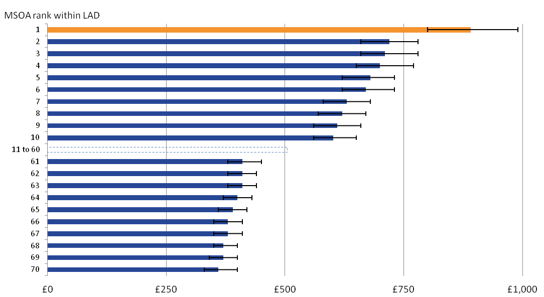
Figure 13 shows the mean net weekly household income (equivalised) AHC (with 95% confidence intervals) for the 23 MSOAs in South Tyneside local authority district (LAD). This LAD had the largest proportion of MSOAs with estimates that were significantly lower than the MSOA that had the highest mean total income in the LAD. All of the other 22 MSOAs had significantly lower net income after housing costs.

Figure 13: Mean net weekly household income (equivalised) after housing costs for middle layer super output areas within local authority districts

South Tyneside, 2013/14

Source: Office for National Statistics

Notes:

1. Ranked by highest mean net weekly household income (equivalised) after housing costs.

Download this image Figure 13: Mean net weekly household income (equivalised) after housing costs for middle layer super output areas within local authority districts

.png (13.5 kB) .xls (28.7 kB)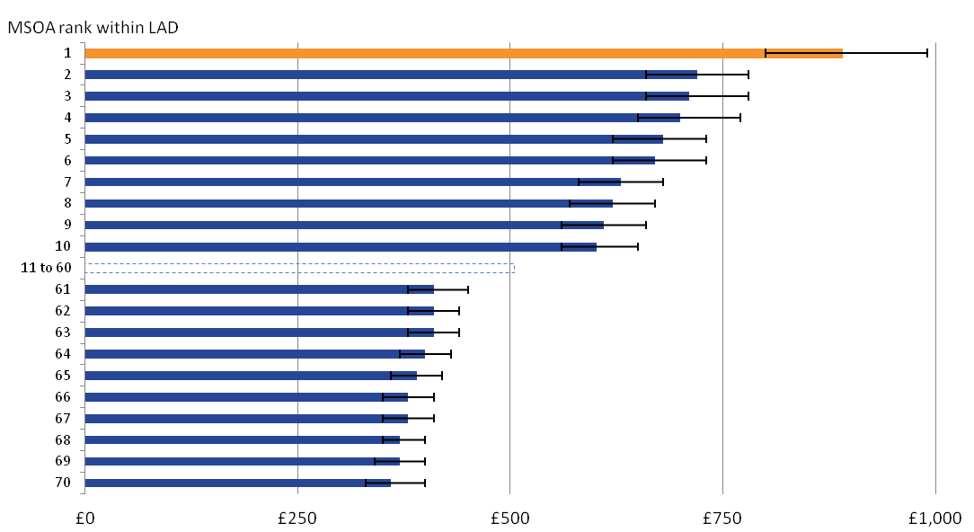

There were other LADs containing a similarly high proportion of MSOAs with lower net AHC income compared with the highest ranked MSOA. For example, in Basildon 21 out of 22 MSOAs had significantly lower net AHC income compared with the highest MSOA. However, not all LADs show this pattern. Newham contains 37 MSOAs in which none had significantly different net AHC income than the highest ranked MSOA.

Conversely, the LAD with the largest proportion of MSOAs with significantly higher net AHC income than the lowest ranked MSOA is Wycombe (22 out of 23).

Administrative Data Census Research Outputs: Income from PAYE and benefits for tax year ending 2014.

Plans for the future development of the small area income estimates.

Household disposable income and inequality.

This release provides new estimates of mean weekly household income for 2013/14 (the financial year ending March 2014) for middle layer super output areas (MSOAs) in England and Wales.

This publication also provides the data and technical report for the 2011/12 households in poverty estimates for MSOAs in England and Wales. These provide modelled estimates of the proportion of households in each MSOA with an income lower than 60% of the national median.

We will produce the 2015/16 small area incomes in 2017 using the method used to produce these estimates. Alongside this, we will also investigate the use of more administrative data to improve the quality of the modelled estimates, explore new methods of estimating household income and report our findings.

For more information about the quality and methods used to produce these statistics, see our technical report.