1. Main points
Extending the open-ended final age group interval from 85 and over to 90 and over resulted in greater accuracy of life expectancy estimates across all age groups.
The point estimate of life expectancy tended to be slightly lower when life tables were closed at 90 and over compared with 85 and over.
The inclusion of a variance term in the final age group of the 90 and over abridged life tables resulted in increased standard errors (SEs) and relatively less precise estimates in all age groups compared with the 85 and over life tables.
Standard errors and relative standard errors (RSEs) were higher under the 90 and over than the 85 and over life tables; however, in both cases, the RSEs in all age groups and across all geographical levels were lower than 5%, demonstrating that estimates under both life tables are reliable.
In England, the difference in life expectancy between the 85 and over and 90 and over life tables were statistically significant in all age groups. Conversely, there was no significant difference in life expectancy between the 85 and over and 90 and over life tables in Wales.
In most regions, significant differences in life expectancy between the 85 and over and 90 and over life tables tended to be at older ages. At birth, significant differences were observed in London only. At age 65, significant differences were found for men in the East of England, London, South East and South West, and for women in London.
Despite shifts in the point estimate of local area life expectancy between the 85 and over and 90 and over life tables, the only significant differences observed across all age groups were in Brent and Westminster, where 80- to 84-year-old women had significantly lower life expectancy when the life tables were closed at 90 and over.
The differences in life expectancy between the 85 and over and 90 and over life tables were statistically significant in the two least deprived fifths of lower super output areas (LSOAs) for males (quintiles 4 and 5), and in the least deprived for females (quintile 5). Conversely, for both sexes there was no significant difference between the comparable life tables for the most deprived fifth of LSOAs (quintile 1). Differences in the other intervening quintiles were mainly significant at older ages.
Back to table of contents2. Introduction
Life expectancy is produced using a statistical tool known as a life table. The most commonly used life table statistic is the average remaining years of life or life expectancy. We produce subnational life expectancy using abridged life table methods. Abridged life tables are based on deaths and population data by age groups (usually 5-year age groups, with an open-ended final age interval).
Abridged life tables are constructed to show the mortality experience of a hypothetical cohort of babies born at the same time, and subject throughout their lifetime to the age-specific mortality rates in a specific area in a given period.
Why is the current open-ended age interval set at 85 years and over?
We have used a consistent life table methodology for many years, which was developed when sub-national population estimates were only available up to 85 and over.
Rationale for extending the open-ended age interval
Abridged life tables assume that deaths are evenly distributed within age groups, so that the probability of dying is the same for all individuals within an age group regardless of their age. However, this assumption becomes increasingly less accurate as the width of age groups increase, as is the case with the open-ended age interval.
The elderly population is a relatively heterogeneous group, consisting of people in different health states. Therefore, the average risk of dying at age 85 and over (as a whole) may not accurately describe the risk of dying in smaller age groups making up this broad age interval. For example, table 1 shows that the mortality patterns at very old ages are obscured when regional life tables are closed at 85 and over. Differences are evident in both the mortality rates and in the population structure within the 85 and over age interval in each English region, as less than a third of men and less than half of women in this age group were aged 90 years or older (90 and over hereafter).
The differing population structures also meant the mortality rates in the 85 and over population aligned more closely with those in the 85 to 89 years age group than the 90 and over population (table 1).
Table 1: Age-specific mortality rates among those aged 85 and over, regions of England, 2012 to 2014
| Mortality rate | |||||||
| Sex | Region | 85-89 | 90+ | 85+ | % of 85+ population who are 90 and over | ||
| Male | North East | 0.14 | 0.24 | 0.17 | 28 | ||
| North West | 0.13 | 0.24 | 0.17 | 29 | |||
| Yorkshire and The Humber | 0.14 | 0.24 | 0.17 | 29 | |||
| East Midlands | 0.14 | 0.24 | 0.17 | 30 | |||
| West Midlands | 0.13 | 0.24 | 0.16 | 29 | |||
| East of England | 0.12 | 0.24 | 0.16 | 30 | |||
| London | 0.11 | 0.2 | 0.14 | 31 | |||
| South East | 0.12 | 0.23 | 0.16 | 32 | |||
| South West | 0.12 | 0.24 | 0.16 | 32 | |||
| Female | North East | 0.11 | 0.22 | 0.15 | 37 | ||
| North West | 0.11 | 0.21 | 0.15 | 38 | |||
| Yorkshire and The Humber | 0.11 | 0.22 | 0.15 | 38 | |||
| East Midlands | 0.1 | 0.21 | 0.14 | 39 | |||
| West Midlands | 0.1 | 0.2 | 0.14 | 39 | |||
| East of England | 0.09 | 0.2 | 0.14 | 40 | |||
| London | 0.09 | 0.19 | 0.13 | 40 | |||
| South East | 0.09 | 0.2 | 0.14 | 41 | |||
| South West | 0.09 | 0.21 | 0.14 | 41 | |||
| Source: Office for National Statistics | |||||||
Download this table Table 1: Age-specific mortality rates among those aged 85 and over, regions of England, 2012 to 2014
.xls (28.7 kB)Historically, the number of people at older ages has been relatively small. However, due to improvements in survival rates, particularly for the over-65s, there has been a rapid increase in the number of people living to very old ages. For example, the number of people aged 85 years and over in England and Wales increased by 19%, from 1.01 million on Census Day 2001, to 1.25 million in 2011 (ONS, 2013).
The increase in the number of people surviving to older ages is also evident in the life tables for England and Wales. The survivorship curves in Figures 1 and 2 show the improvements in survival for baby boys and girls between the periods 1980 to 1982 and 2012 to 2014. The probability that a newborn baby girl, for example, would survive to reach the age of 85 years increased, from 32% in 1980 to 1982, to 53% in 2012 to 2014. These shifts in survival provide clear evidence for the review of the open-ended age limit currently in use.
Figure 1: Number of survivors (lx) from a hypothetical cohort of 100,000 newborn baby boys, England and Wales, 1980–82 and 2012–14
Source: Office for national statistics - National Life Tables
Download this chart Figure 1: Number of survivors (lx) from a hypothetical cohort of 100,000 newborn baby boys, England and Wales, 1980–82 and 2012–14
Image .csv .xls
Figure 2: Number of survivors (lx) from a hypothetical cohort of 100,000 newborn baby girls, England and Wales, 1980–82 and 2012–14
Source: Office for national statistics - National Life Tables
Download this chart Figure 2: Number of survivors (lx) from a hypothetical cohort of 100,000 newborn baby girls, England and Wales, 1980–82 and 2012–14
Image .csv .xlsNew open-ended age interval
It is desirable to set the new limit for the open-ended age interval as high as possible, so that results from the abridged life tables align as closely as possible with those from complete life tables. However, it may not be possible to do so because of a lack of adequately disaggregated population data at very old ages.
While deaths data are often available by single year of age, allowing for these data to be aggregated using a variety of upper age limits, population data, particularly at subnational levels, are often produced using specific upper age limits (often 85 and over or 90 and over). Consequently, constructing abridged life tables with an open-ended age interval of 95 and over or 100 and over is not currently feasible for local areas. We will therefore aggregate the deaths data to match the age-structure of the available population data and close the abridged life tables at 90 and over. This age group was also recommended by us for the calculation of age-standardised rates in the UK, following the introduction of the 2013 European Standard Population.
Back to table of contents3. Methods
Impact of closing abridged life tables at 90 and over
To assess the impact of extending the open-ended age interval from 85 and over to 90 and over, we compared life expectancy estimates produced using the 85 and over abridged life tables with those based on the 90 and over life tables. We did this for England, Wales, regions of England, local authorities and lower super output areas (LSOAs) grouped into quintiles (fifths), according to the 2015 Indices of Multiple Deprivation (IMD 2015). Specifically we:
- tested the accuracy of the abridged life tables closed at 85 and over and 90 and over at national level for England and Wales by comparing the point estimates of life expectancy in these abridged life tables with the more accurate point estimates in a reference complete life table – the national life tables (NLT)
- included a variance term in the open-ended age group and assessed its impact on SEs and the precision of life expectancy estimates in all age groups
- carried out statistical tests to detect significant differences between life expectancy based on life tables closed at 85 and over and 90 and over
- used relative standard errors (RSEs) to assess the reliability of life expectancy estimates
The headline figures in our sub-national life expectancy release are life expectancy at birth and at age 65, so for ease of reporting the main focus here is on these two age groups.
Variance for the open-ended age group
There is widespread interest in life expectancy at very old ages, but in order to compare two life expectancy estimates, for example, over time or between two local areas, statistical tests need to be carried out. One way of doing this is to calculate standard errors (SEs) and confidence intervals for life expectancy estimates to exclude the role of chance as a likely explanation for differences between areas and over time.
In the Chiang II method, which we use in constructing abridged life tables, the variance of life expectancy is a function of the probability of survival. Therefore, SEs and associated confidence intervals are calculated for every age group, apart from the final. Since everyone in the life table eventually dies, the probability of survival in the final age interval is zero and, by definition, the variance in this age group is also zero. In practice, this means that it is not possible to calculate SEs and confidence intervals for the final age group using Chiang’s method.
Conversely, Silcocks, Jenna and Reza (2001) argue that the variance in the final age group is a function of the mean length of survival (expressed as the notional width of the final age interval), not the probability of survival. Their method therefore enables computation of SEs and confidence intervals for the final age group using the assumption of a Poisson distribution for deaths occurring in the final age group.
To ensure that inferences about the expectation of life can be made in all age groups, we will combine the Chiang II abridged life table methods, which we currently use, with Silcocks’ method. Specifically, we will continue to calculate life expectancy and confidence intervals for each age group up to 85 to 89 years using the Chiang II abridged life table methods, and we will incorporate Silcocks’ method of estimating the variance of life expectancy in the open-ended age group in order to calculate the confidence intervals for the 90 and over age group.
Test for difference between life expectancy based on 85 and over and 90 and over life tables
To determine whether or not the difference between life expectancy based on the 85 and over and 90 and over life tables was significant, we calculated z-scores and the probability (p-value) of obtaining a value as extreme as the z-statistic (see table 2).
If the value of the z-score is greater than or equal to 1.96 (or less than or equal to negative 1.96), the critical value of a two-tailed test at the 95% level, the difference between the two life expectancy estimates being tested is statistically significant. If the difference is greater than negative 1.96 and less than 1.96 (inclusive) then the difference is not statistically significant.
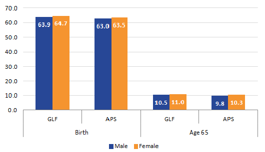
The z-score for testing the equality of life expectancy under both life tables was calculated as:
Equation 1
Notes:
Where:
LE1i is the life expectancy in age group i, based on life tables closed at 85+
LE2i is the life expectancy in age group i, based on life tables closed at 90+
SE is the standard error of life expectancy in age group i
Download this image Equation 1
.png (2.1 kB)
Assessing the reliability of life expectancy estimates
The random variation in the number of deaths in each year means that the mortality rates used in constructing life tables are made up of a certain level of uncertainty (measured as standard errors).
To assess the impact of this uncertainty on the stability and reliability of life expectancy estimates, we calculated relative standard errors. In simple terms, the measurement (life expectancy) could be thought of as the ‘signal’ while the uncertainty around it (standard error) represents the “noise”. The higher the RSE, the more unstable and less reliable the life expectancy estimate is. Estimates with RSEs of up to 25% are thought to be reliable (ABS, 2010, CDC, 2010).
The RSE is calculated as the SE (noise) of life expectancy divided by the life expectancy estimate itself (signal), expressed as a percentage:
Equation 2

Notes:
Where:
SEi is the standard error of life expectancy in age group i
LEi is the life expectancy in age group i
Download this image Equation 2
.png (958 B)
4. Results
Comparisons drawn between life tables constructed using the open-ended age groups of 85 and over and 90 and over are for age-specific life expectancy up to age group 80 to 84 years. Age groups 85 to 89, 85 and over and 90 and over are not common to both sets of life tables, so it is not possible to assess differences for these age groups.
England and Wales
There was closer agreement between life expectancy estimates in the 90 and over abridged life tables and the national life tables (NLTs) than there was between the 85 and over life tables and the NLTs, demonstrating that life expectancy is more accurate when the life tables are closed at 90 and over (table 2). However, the inclusion of a variance term in the final age group of the 90 and over abridged life tables resulted in increased SEs and reduced precision for these estimates in all age groups.
In England, the computed z-score for every age group was greater than 1.96, demonstrating that the differences between 85 and over and 90 and over English life tables were statistically significant. The opposite was true in Wales, where there was no significant difference in life expectancy between the 85 and over and 90 and over life tables.
Tables 2 and 3 show the significance test results for male and female life expectancy at birth and at age 65.
Table 2: Significance test for difference between life expectancy at birth, based on life tables closed at 85 and over and 90 and over, England and Wales, 2012 to 2014
| Sex | Country | Life tables closed at 85+ | Life tables closed at 90+ | z-score | p-value | Significant difference | ||||
| LE at birth | Lower 95% CI | Upper 95% CI | LE at birth | Lower 95% CI | Upper 95% CI | |||||
| Male | England and Wales | 79.44 | 79.41 | 79.47 | 79.34 | 79.31 | 79.36 | 3.62 | 0.00 | Yes |
| England | 79.55 | 79.52 | 79.57 | 79.44 | 79.41 | 79.47 | 3.59 | 0.00 | Yes | |
| Wales | 78.51 | 78.39 | 78.63 | 78.42 | 78.30 | 78.55 | 0.69 | 0.49 | No | |
| Female | England and Wales | 83.11 | 83.09 | 83.14 | 83.03 | 83.01 | 83.06 | 2.96 | 0.00 | Yes |
| England | 83.20 | 83.17 | 83.22 | 83.11 | 83.09 | 83.14 | 3.00 | 0.00 | Yes | |
| Wales | 82.35 | 82.24 | 82.46 | 82.30 | 82.19 | 82.42 | 0.37 | 0.71 | No | |
| Source: Office for national statistics | ||||||||||
Download this table Table 2: Significance test for difference between life expectancy at birth, based on life tables closed at 85 and over and 90 and over, England and Wales, 2012 to 2014
.xls (28.2 kB)
Table 3: Significance test for difference between life expectancy at age 65 based on life tables closed at 85 and over and 90 and over, England and Wales, 2012 to 2014
| Sex | Country | Life tables closed at 85+ | Life tables closed at 90+ | z-score | p-value | Significant difference | ||||
| LE at age 65 | Lower 95% CI | Upper 95% CI | LE at age 65 | Lower 95% CI | Upper 95% CI | |||||
| Male | England and Wales | 18.72 | 18.70 | 18.74 | 18.60 | 18.58 | 18.62 | 6.14 | 0.00 | Yes |
| England | 18.77 | 18.75 | 18.79 | 18.65 | 18.63 | 18.67 | 6.04 | 0.00 | Yes | |
| Wales | 18.19 | 18.12 | 18.26 | 18.09 | 18.01 | 18.17 | 1.29 | 0.20 | No | |
| Female | England and Wales | 21.14 | 21.12 | 21.16 | 21.05 | 21.03 | 21.07 | 4.63 | 0.00 | Yes |
| England | 21.19 | 21.17 | 21.21 | 21.10 | 21.08 | 21.12 | 4.66 | 0.00 | Yes | |
| Wales | 20.60 | 20.53 | 20.66 | 20.55 | 20.47 | 20.63 | 0.62 | 0.53 | No | |
| Source: Office for national statistics | ||||||||||
Download this table Table 3: Significance test for difference between life expectancy at age 65 based on life tables closed at 85 and over and 90 and over, England and Wales, 2012 to 2014
.xls (28.2 kB)The impact on standard errors of extending the open-ended age interval to 90 and over was more pronounced at older ages. The percentage difference in SEs between the 85 and over and 90 and over life tables increased with age, ranging from 3% at birth to 32% in age group 80 to 84 for males in England. The comparable increase for females was from 5% at birth to 35% in age group 80 to 84. A similar pattern was observed in Wales. The increased standard errors meant that confidence intervals were generally wider under the 90 and over life tables, but the increase was slightly greater at older than at younger ages.
Although estimates of life expectancy were less precise under the 90 and over open-ended life tables, the RSE was relatively low in both the 85 and over and 90 and over abridged life tables. The RSE tended to increase with age and was higher in Wales than in England. Nevertheless, it was less than 0.5% in all age groups in both countries, indicating that estimates under both life tables are reliable.
Table 4: Standard errors (SE) and relative standard errors (RSE) for life expectancy at birth, based on life tables closed at 85 and over and 90 and over, England and Wales, 2012 to 2014
| Life tables closed at 85+ | Life tables closed at 90+ | ||||||
| Sex | Country | LE at birth | SE(LE) | RSE (%) | LE at birth | SE(LE) | RSE (%) |
| Male | England and Wales | 79.44 | 0.014 | 0.02 | 79.34 | 0.015 | 0.02 |
| England | 79.55 | 0.015 | 0.02 | 79.44 | 0.015 | 0.02 | |
| Wales | 78.51 | 0.061 | 0.08 | 78.42 | 0.063 | 0.08 | |
| Female | England and Wales | 83.11 | 0.013 | 0.02 | 83.03 | 0.014 | 0.02 |
| England | 83.2 | 0.013 | 0.02 | 83.11 | 0.014 | 0.02 | |
| Wales | 82.35 | 0.056 | 0.07 | 82.3 | 0.058 | 0.07 | |
| Source: Office for National Statistics | |||||||
Download this table Table 4: Standard errors (SE) and relative standard errors (RSE) for life expectancy at birth, based on life tables closed at 85 and over and 90 and over, England and Wales, 2012 to 2014
.xls (27.6 kB)
Table 5: Standard errors (SE) and relative standard errors (RSE) for life expectancy at age 65, based on life tables closed at 85 and over and 90 and over, England and Wales, 2012 to 2014
| Life tables closed at 85+ | Life tables closed at 90+ | ||||||
| Sex | Country | LE at age 65 | SE(LE) | RSE (%) | LE at age 65 | SE(LE) | RSE (%) |
| Male | England and Wales | 18.72 | 0.01 | 0.05 | 18.60 | 0.01 | 0.06 |
| England | 18.77 | 0.01 | 0.05 | 18.65 | 0.01 | 0.06 | |
| Wales | 18.19 | 0.04 | 0.20 | 18.09 | 0.04 | 0.22 | |
| Female | England and Wales | 21.14 | 0.01 | 0.04 | 21.05 | 0.01 | 0.05 |
| England | 21.19 | 0.01 | 0.04 | 21.10 | 0.01 | 0.05 | |
| Wales | 20.60 | 0.04 | 0.17 | 20.55 | 0.04 | 0.20 | |
| Source: Office for National Statistics | |||||||
Download this table Table 5: Standard errors (SE) and relative standard errors (RSE) for life expectancy at age 65, based on life tables closed at 85 and over and 90 and over, England and Wales, 2012 to 2014
.xls (27.6 kB)Regions of England
The patterns found at national level were also evident in English regions, with abridged life tables closed at 90 and over producing more accurate point estimates of life expectancy than those based on 85 and over.
In most regions, significant differences in life expectancy between the 85 and over and 90 and over life tables tended to be at older ages. In some regions, significant differences were observed from relatively young age groups onwards. For example, the difference in male life expectancy in the South East between the 85 and over and 90 and over life tables was significant from age group 45 to 49 years onwards. In London, there was no significant difference in sex-specific life expectancy between the 85 and over and 90 and over life tables at any age.
At birth, there was no significant difference in sex-specific life expectancy between the 85 and over and 90 and over life tables for all regions, apart from London where it was significantly lower in the 90 and over life tables.
At age 65, the difference in life expectancy between the 85 and over and 90 and over life tables was significant for men in the East of England, London, South East and South West, and for women in London.
Table 6: Significance test for difference between life expectancy at birth based on life tables closed at 85 and over and 90 and over, English regions, 2012 to 2014
| Life tables closed at 85+ | Life tables closed at 90+ | |||||||||
| Sex | Region | LE at birth | Lower 95% CI | Upper 95% CI | LE at birth | Lower 95% CI | Upper 95% CI | z-score | p-value | Significant difference |
| Male | North East | 78.01 | 77.88 | 78.14 | 77.92 | 77.79 | 78.06 | 0.64 | 0.52 | No |
| North West | 78.12 | 78.04 | 78.2 | 78.03 | 77.95 | 78.12 | 1.04 | 0.3 | No | |
| Yorkshire and The Humber | 78.7 | 78.6 | 78.79 | 78.62 | 78.53 | 78.71 | 0.81 | 0.42 | No | |
| East Midlands | 79.38 | 79.28 | 79.48 | 79.29 | 79.19 | 79.39 | 0.85 | 0.4 | No | |
| West Midlands | 78.86 | 78.77 | 78.95 | 78.76 | 78.67 | 78.85 | 1.09 | 0.28 | No | |
| East of England | 80.44 | 80.36 | 80.52 | 80.31 | 80.22 | 80.4 | 1.5 | 0.13 | No | |
| London | 80.33 | 80.25 | 80.41 | 80.15 | 80.07 | 80.24 | 2.1 | 0.04 | Yes | |
| South East | 80.55 | 80.48 | 80.62 | 80.44 | 80.36 | 80.51 | 1.58 | 0.11 | No | |
| South West | 80.21 | 80.12 | 80.3 | 80.11 | 80.02 | 80.2 | 1.12 | 0.26 | No | |
| Female | North East | 81.68 | 81.56 | 81.8 | 81.62 | 81.49 | 81.74 | 0.49 | 0.62 | No |
| North West | 81.86 | 81.78 | 81.93 | 81.8 | 81.72 | 81.88 | 0.73 | 0.47 | No | |
| Yorkshire and The Humber | 82.38 | 82.29 | 82.46 | 82.33 | 82.24 | 82.42 | 0.55 | 0.58 | No | |
| East Midlands | 83.05 | 82.96 | 83.14 | 82.95 | 82.86 | 83.05 | 0.97 | 0.33 | No | |
| West Midlands | 82.86 | 82.78 | 82.95 | 82.77 | 82.69 | 82.86 | 1.02 | 0.31 | No | |
| East of England | 83.79 | 83.71 | 83.87 | 83.69 | 83.61 | 83.77 | 1.24 | 0.21 | No | |
| London | 84.2 | 84.13 | 84.27 | 84.01 | 83.93 | 84.09 | 2.48 | 0.01 | Yes | |
| South East | 84.01 | 83.94 | 84.07 | 83.94 | 83.87 | 84.01 | 0.98 | 0.32 | No | |
| South West | 83.95 | 83.87 | 84.03 | 83.88 | 83.79 | 83.96 | 0.83 | 0.41 | No | |
| Source: Office for National Statistics | ||||||||||
Download this table Table 6: Significance test for difference between life expectancy at birth based on life tables closed at 85 and over and 90 and over, English regions, 2012 to 2014
.xls (29.2 kB)
Table 7: Significance test for difference between life expectancy at age 65 based on life tables closed at 85 and over and 90 and over, English regions, 2012 to 2014
| Life tables closed at 85+ | Life tables closed at 90+ | |||||||||
| Sex | Region | LE at age 65 | Lower 95% CI | Upper 95% CI | LE at age 65 | Lower 95% CI | Upper 95% CI | z-score | p-value | Significant difference |
| Male | North East | 17.9 | 17.8 | 18.0 | 17.8 | 17.7 | 17.9 | 1.2 | 0.2 | No |
| North West | 18.0 | 17.9 | 18.0 | 17.9 | 17.8 | 17.9 | 1.9 | 0.1 | No | |
| Yorkshire and The Humber | 18.2 | 18.1 | 18.2 | 18.1 | 18.0 | 18.2 | 1.4 | 0.2 | No | |
| East Midlands | 18.6 | 18.5 | 18.6 | 18.5 | 18.4 | 18.6 | 1.5 | 0.1 | No | |
| West Midlands | 18.5 | 18.4 | 18.6 | 18.4 | 18.3 | 18.4 | 1.9 | 0.1 | No | |
| East of England | 19.3 | 19.3 | 19.4 | 19.2 | 19.1 | 19.2 | 2.5 | 0.0 | Yes | |
| London | 19.2 | 19.2 | 19.3 | 19.0 | 19.0 | 19.1 | 3.0 | 0.0 | Yes | |
| South East | 19.3 | 19.3 | 19.4 | 19.2 | 19.1 | 19.3 | 2.6 | 0.0 | Yes | |
| South West | 19.3 | 19.2 | 19.4 | 19.2 | 19.1 | 19.2 | 2.0 | 0.0 | Yes | |
| Female | North East | 20.0 | 20.0 | 20.1 | 20.0 | 19.9 | 20.1 | 0.8 | 0.4 | No |
| North West | 20.3 | 20.2 | 20.3 | 20.2 | 20.1 | 20.3 | 1.2 | 0.2 | No | |
| Yorkshire and The Humber | 20.6 | 20.5 | 20.6 | 20.5 | 20.4 | 20.6 | 0.9 | 0.4 | No | |
| East Midlands | 21.1 | 21.0 | 21.1 | 21.0 | 20.9 | 21.0 | 1.6 | 0.1 | No | |
| West Midlands | 21.1 | 21.0 | 21.1 | 21.0 | 20.9 | 21.0 | 1.7 | 0.1 | No | |
| East of England | 21.6 | 21.6 | 21.6 | 21.5 | 21.4 | 21.6 | 1.9 | 0.1 | No | |
| London | 21.9 | 21.9 | 22.0 | 21.7 | 21.7 | 21.8 | 3.3 | 0.0 | Yes | |
| South East | 21.8 | 21.7 | 21.8 | 21.7 | 21.6 | 21.7 | 1.5 | 0.1 | No | |
| South West | 21.8 | 21.7 | 21.8 | 21.7 | 21.6 | 21.8 | 1.4 | 0.2 | No | |
| Source: Office for National Statistics | ||||||||||
Download this table Table 7: Significance test for difference between life expectancy at age 65 based on life tables closed at 85 and over and 90 and over, English regions, 2012 to 2014
.xls (29.7 kB)The inclusion of a variance term in the final age group of the 90+ regional life tables resulted in increased SEs and relatively less precise estimates in all age groups compared with the 85 and over life tables.
The percentage increase in SEs between the 85 and over and 90 and over regional life tables increased with age and was greater for females than males. In each life table type, the magnitude of the SE in each age group was generally greater in the north than in the south of England; however, the increase in SEs between the two life tables tended to be greater in southern regions.
SEs and RSEs were higher under the 90 and over than the 85 and over life tables; however in both cases, the RSEs were lower than 1% in all age groups, demonstrating that estimates under both life tables are reliable.
Table 8: Standard errors (SE) and relative standard errors (RSE) for life expectancy at birth, based on life tables closed at 85 and over and 90 and over, region of England, to 2014
| Life tables closed at 85+ | Life tables closed at 90+ | ||||||
| Sex | Region | LE at birth | SE(LE) | RSE (%) | LE at birth | SE(LE) | RSE (%) |
| Male | North East | 78.0 | 0.1 | 0.1 | 77.9 | 0.1 | 0.1 |
| North West | 78.1 | 0.0 | 0.1 | 78.0 | 0.0 | 0.1 | |
| Yorkshire and The Humber | 78.7 | 0.1 | 0.1 | 78.6 | 0.1 | 0.1 | |
| East Midlands | 79.4 | 0.1 | 0.1 | 79.3 | 0.1 | 0.1 | |
| West Midlands | 78.9 | 0.1 | 0.1 | 78.8 | 0.1 | 0.1 | |
| East of England | 80.4 | 0.0 | 0.1 | 80.3 | 0.0 | 0.1 | |
| London | 80.3 | 0.0 | 0.1 | 80.2 | 0.0 | 0.1 | |
| South East | 80.5 | 0.0 | 0.0 | 80.4 | 0.0 | 0.1 | |
| South West | 80.2 | 0.1 | 0.1 | 80.1 | 0.1 | 0.1 | |
| Female | North East | 81.7 | 0.1 | 0.1 | 81.6 | 0.1 | 0.1 |
| North West | 81.9 | 0.0 | 0.0 | 81.8 | 0.0 | 0.0 | |
| Yorkshire and The Humber | 82.4 | 0.0 | 0.1 | 82.3 | 0.1 | 0.1 | |
| East Midlands | 83.0 | 0.1 | 0.1 | 83.0 | 0.1 | 0.1 | |
| West Midlands | 82.9 | 0.0 | 0.1 | 82.8 | 0.0 | 0.1 | |
| East of England | 83.8 | 0.0 | 0.1 | 83.7 | 0.0 | 0.1 | |
| London | 84.2 | 0.0 | 0.0 | 84.0 | 0.0 | 0.1 | |
| South East | 84.0 | 0.0 | 0.0 | 83.9 | 0.0 | 0.0 | |
| South West | 84.0 | 0.0 | 0.0 | 83.9 | 0.0 | 0.1 | |
| Source: Office for National Statistics | |||||||
Download this table Table 8: Standard errors (SE) and relative standard errors (RSE) for life expectancy at birth, based on life tables closed at 85 and over and 90 and over, region of England, to 2014
.xls (28.7 kB)
Table 9: Standard errors (SE) and relative standard errors (RSE) for life expectancy at age 65, based on life tables closed at 85 and over and 90 and over, region of England, 2012 to 2014
| Life tables closed at 85+ | Life tables closed at 90+ | ||||||
| Sex | Region | LE at age 65 | SE(LE) | RSE (%) | LE at age 65 | SE(LE) | RSE (%) |
| Male | North East | 17.9 | 0.0 | 0.2 | 17.8 | 0.0 | 0.3 |
| North West | 18.0 | 0.0 | 0.1 | 17.9 | 0.0 | 0.2 | |
| Yorkshire and The Humber | 18.2 | 0.0 | 0.2 | 18.1 | 0.0 | 0.2 | |
| East Midlands | 18.6 | 0.0 | 0.2 | 18.5 | 0.0 | 0.2 | |
| West Midlands | 18.5 | 0.0 | 0.2 | 18.4 | 0.0 | 0.2 | |
| East of England | 19.3 | 0.0 | 0.1 | 19.2 | 0.0 | 0.2 | |
| London | 19.2 | 0.0 | 0.2 | 19.0 | 0.0 | 0.2 | |
| South East | 19.3 | 0.0 | 0.1 | 19.2 | 0.0 | 0.1 | |
| South West | 19.3 | 0.0 | 0.1 | 19.2 | 0.0 | 0.2 | |
| Female | North East | 20.0 | 0.0 | 0.2 | 20.0 | 0.0 | 0.2 |
| North West | 20.3 | 0.0 | 0.1 | 20.2 | 0.0 | 0.1 | |
| Yorkshire and The Humber | 20.6 | 0.0 | 0.1 | 20.5 | 0.0 | 0.1 | |
| East Midlands | 21.1 | 0.0 | 0.1 | 21.0 | 0.0 | 0.2 | |
| West Midlands | 21.1 | 0.0 | 0.1 | 21.0 | 0.0 | 0.1 | |
| East of England | 21.6 | 0.0 | 0.1 | 21.5 | 0.0 | 0.1 | |
| London | 21.9 | 0.0 | 0.1 | 21.7 | 0.0 | 0.2 | |
| South East | 21.8 | 0.0 | 0.1 | 21.7 | 0.0 | 0.1 | |
| South West | 21.8 | 0.0 | 0.1 | 21.7 | 0.0 | 0.1 | |
| Source: Office for National Statistics | |||||||
Download this table Table 9: Standard errors (SE) and relative standard errors (RSE) for life expectancy at age 65, based on life tables closed at 85 and over and 90 and over, region of England, 2012 to 2014
.xls (28.7 kB)Area deprivation quintiles
As with other geographical levels examined, estimates of life expectancy were more accurate, but less precise when life tables for Indices of Multiple Deprivation (IMD) 2015 quintiles of lower super output areas (LSOAs) were closed at 90 and over as opposed to 85 and over.
For males, there were significant differences in age-specific life expectancy between the 85 and over and 90 and over life tables for the two least deprived fifths of LSOAs (quintiles 4 and 5). In quintiles 2 and 3, significant differences were mainly observed at older ages, while there was no significant difference between the two types of life tables in the most deprived fifth of LSOAs (quintile 1).
For females, significant differences in life expectancy between the 85 and over and 90 and over life tables were also observed in the least deprived fifth of LSOAs, and at older ages in intervening quintiles 2, 3 and 4. As with males, there was no significant difference in life expectancy in the most deprived fifth of LSOAs between the two types of life tables.
Table 10 shows the differences in quintile life expectancy at birth between the 85 and over and 90 and over life tables were significant in the two least deprived quintiles for males and in the least deprived for females. At age 65, significant differences were observed in the three least deprived quintiles for men and in the two least deprived for women (table 11).
Table 10: Significance test for difference between life expectancy at birth based on life tables closed at 85 and over and 90 and over, IMD 2015 quintile of LSOA, 2012 to 2014
| Life tables closed at 85+ | Life tables closed at 90+ | |||||||||
| Sex | IMD 2015 quintile | LE at birth | Lower 95% CI | Upper 95% CI | LE at birth | Lower 95% CI | Upper 95% CI | z-score | p-value | Significant difference |
| Male | 1 - Most deprived | 75.07 | 75 | 75.14 | 75.04 | 74.97 | 75.11 | 0.43 | 0.665 | No |
| 2 | 78.18 | 78.12 | 78.25 | 78.12 | 78.05 | 78.18 | 1.01 | 0.314 | No | |
| 3 | 80.04 | 79.98 | 80.1 | 79.95 | 79.88 | 80.01 | 1.44 | 0.149 | No | |
| 4 | 81.31 | 81.25 | 81.37 | 81.17 | 81.11 | 81.23 | 2.27 | 0.023 | Yes | |
| 5 - Least deprived | 82.75 | 82.69 | 82.81 | 82.51 | 82.45 | 82.58 | 3.71 | 0.000 | Yes | |
| Female | 1 - Most deprived | 79.77 | 79.7 | 79.84 | 79.74 | 79.67 | 79.81 | 0.41 | 0.679 | No |
| 2 | 82.1 | 82.04 | 82.16 | 82.05 | 81.99 | 82.12 | 0.76 | 0.445 | No | |
| 3 | 83.48 | 83.43 | 83.54 | 83.43 | 83.36 | 83.49 | 0.99 | 0.323 | No | |
| 4 | 84.43 | 84.38 | 84.49 | 84.35 | 84.29 | 84.4 | 1.46 | 0.145 | No | |
| 5 - Least deprived | 85.73 | 85.67 | 85.78 | 85.49 | 85.43 | 85.56 | 3.92 | 0.000 | Yes | |
| Source: Office for national statistics | ||||||||||
Download this table Table 10: Significance test for difference between life expectancy at birth based on life tables closed at 85 and over and 90 and over, IMD 2015 quintile of LSOA, 2012 to 2014
.xls (28.7 kB)
Table 11: Significance test for difference between life expectancy at age 65 based on life tables closed at 85 and over and 90 and over, IMD 2015 quintile of LSOA, 2012 to 2014
| Life tables closed at 85+ | Life tables closed at 90+ | |||||||||
| Sex | IMD 2015 quintile | LE at age 65 | Lower 95% CI | Upper 95% CI | LE at age 65 | Lower 95% CI | Upper 95% CI | z-score | p-value | Significant difference |
| Male | 1 - Most deprived | 16.25 | 16.2 | 16.3 | 16.21 | 16.16 | 16.26 | 0.78 | 0.436 | No |
| 2 | 17.82 | 17.78 | 17.87 | 17.75 | 17.7 | 17.79 | 1.67 | 0.094 | No | |
| 3 | 18.86 | 18.82 | 18.9 | 18.76 | 18.71 | 18.8 | 2.41 | 0.016 | Yes | |
| 4 | 19.62 | 19.59 | 19.66 | 19.47 | 19.42 | 19.51 | 3.71 | 0.000 | Yes | |
| 5 - Least deprived | 20.57 | 20.53 | 20.61 | 20.32 | 20.27 | 20.37 | 5.8 | 0.000 | Yes | |
| Female | 1 - Most deprived | 19.01 | 18.96 | 19.05 | 18.97 | 18.92 | 19.02 | 0.66 | 0.511 | No |
| 2 | 20.39 | 20.35 | 20.43 | 20.34 | 20.29 | 20.38 | 1.17 | 0.241 | No | |
| 3 | 21.26 | 21.22 | 21.3 | 21.2 | 21.15 | 21.24 | 1.54 | 0.125 | No | |
| 4 | 21.86 | 21.82 | 21.89 | 21.77 | 21.72 | 21.81 | 2.24 | 0.025 | Yes | |
| 5 - Least deprived | 22.89 | 22.86 | 22.93 | 22.65 | 22.6 | 22.69 | 5.89 | 0.000 | Yes | |
| Source: Office for national statistics | ||||||||||
Download this table Table 11: Significance test for difference between life expectancy at age 65 based on life tables closed at 85 and over and 90 and over, IMD 2015 quintile of LSOA, 2012 to 2014
.xls (28.7 kB)The inclusion of a variance term in the final age group of the 90 and over quintile life tables resulted in increased SEs and relatively less precise estimates in all age groups compared with the 85 and over life tables. The percentage increase in SEs between the 85 and over and 90 and over regional life tables increased with age and was greater for females than males. Consequently, the increase in confidence interval width was slightly greater at older than at younger ages.
In both the 85 and over and 90 and over life tables, the SE tended to increase with area deprivation. Conversely, the percentage increase in SEs between the two life tables tended to increase as area deprivation decreased.
SEs and RSEs were higher under the 90 and over than the 85 and over life tables; however in both cases, the RSEs were lower than 0.3% in all age groups, demonstrating that estimates under both life tables are reliable.
Table 12: Standard errors (SE) and relative standard errors (RSE) for life expectancy at birth, based on life tables closed at 85 and over and 90 and over, England and Wales, 2012 to 2014
| Life tables closed at 85+ | Life tables closed at 90+ | ||||||
| Sex | IMD 2015 quintile | LE at birth | SE(LE) | RSE (%) | LE at birth | SE(LE) | RSE (%) |
| Male | 1 - Most deprived | 75.1 | 0.03 | 0.05 | 75 | 0.04 | 0.05 |
| 2 | 78.2 | 0.03 | 0.04 | 78.1 | 0.03 | 0.04 | |
| 3 | 80 | 0.03 | 0.04 | 79.9 | 0.03 | 0.04 | |
| 4 | 81.3 | 0.03 | 0.04 | 81.2 | 0.03 | 0.04 | |
| 5 - Least deprived | 82.7 | 0.03 | 0.04 | 82.5 | 0.03 | 0.04 | |
| Female | 1 - Most deprived | 79.8 | 0.03 | 0.04 | 79.7 | 0.03 | 0.04 |
| 2 | 82.1 | 0.03 | 0.04 | 82.1 | 0.03 | 0.04 | |
| 3 | 83.5 | 0.03 | 0.03 | 83.4 | 0.03 | 0.04 | |
| 4 | 84.4 | 0.03 | 0.03 | 84.3 | 0.03 | 0.04 | |
| 5 - Least deprived | 85.7 | 0.03 | 0.03 | 85.5 | 0.03 | 0.04 | |
| Source: Office for national statistics | |||||||
Download this table Table 12: Standard errors (SE) and relative standard errors (RSE) for life expectancy at birth, based on life tables closed at 85 and over and 90 and over, England and Wales, 2012 to 2014
.xls (28.2 kB)
Table 13: Standard errors (SE) and relative standard errors (RSE) for life expectancy at age 65, based on life tables closed at 85 and over and 90 and over, England and Wales, 2012 to 2014
| Life tables closed at 85+ | Life tables closed at 90+ | ||||||
| Sex | IMD 2015 quintile | LE at age 65 | SE(LE) | RSE (%) | LE at age 65 | SE(LE) | RSE (%) |
| Male | 1 - Most deprived | 16.20 | 0.02 | 0.15 | 16.20 | 0.03 | 0.16 |
| 2 | 17.80 | 0.02 | 0.13 | 17.70 | 0.02 | 0.14 | |
| 3 | 18.90 | 0.02 | 0.11 | 18.80 | 0.02 | 0.12 | |
| 4 | 19.60 | 0.02 | 0.10 | 19.50 | 0.02 | 0.12 | |
| 5 - Least deprived | 20.60 | 0.02 | 0.10 | 20.30 | 0.02 | 0.12 | |
| Female | 1 - Most deprived | 19.00 | 0.02 | 0.12 | 19.00 | 0.03 | 0.13 |
| 2 | 20.40 | 0.02 | 0.11 | 20.30 | 0.02 | 0.12 | |
| 3 | 21.30 | 0.02 | 0.09 | 21.20 | 0.02 | 0.11 | |
| 4 | 21.90 | 0.02 | 0.09 | 21.80 | 0.02 | 0.10 | |
| 5 - Least deprived | 22.90 | 0.02 | 0.08 | 22.60 | 0.02 | 0.10 | |
| Source: Office for national statistics | |||||||
Download this table Table 13: Standard errors (SE) and relative standard errors (RSE) for life expectancy at age 65, based on life tables closed at 85 and over and 90 and over, England and Wales, 2012 to 2014
.xls (28.2 kB)Local authorities
As with higher level geographies, the point estimates of life expectancy at local authority level were more accurate, but less precise when the life tables were closed at 90 and over compared with 85 and over. In the majority of local authorities, the point estimate of life expectancy was lower when the life tables were closed at 90 and over compared with 85 and over, but in some cases it was higher.
At local authority level, the impact of extending the open-ended age group from 85 and over to 90 and over was relatively small. For males, the difference in the point estimate of life expectancy at birth, between the 85 and over and 90 and over life tables, ranged from a loss of 0.03 years in Watford, to an increase of 0.4 years in Camden. For females at birth, it ranged from a loss of 0.1 years in Surrey Heath to an increase of 0.6 years in Broxbourne. Similar shifts in the point estimate were also found in these areas at age 65.
In England and Wales, 97% (337 out of 346) of local authorities for males and 87% (300 out of the 346) for females saw a small decrease in the point estimate of life expectancy at birth. Again, similar proportions were observed at age 65.
Despite these shifts in the point estimate, there was no significant difference in life expectancy at birth and at age 65 between the 85 and over and 90 and over local authority life tables. Across all age groups, the only significantly differences observed were in Brent and Westminster, where life expectancy among 80 to 84-year-old females were significantly lower when the life tables were closed at 90 and over compared with 85 and over.
The inclusion of a variance term in the open-ended age interval meant that SEs were higher in the 90 and over life tables for local authorities compared with the 85 and over tables. Consequently, confidence intervals were also wider in the 90 and over life tables. Nevertheless, the impact of the additional variance term was small, resulting in a loss of precision (as measured by the increase in confidence interval width) ranging from 0.01 years in Manchester, to 0.2 years in Westminster for males at birth. The corresponding loss of precision for females at birth ranged from 0.02 years in County Durham to 0.2 years in Camden.
At age 65, the loss of precision ranged from 0.02 years in Manchester, to 0.4 years in Westminster and for females, from 0.03 years in Leeds, to 0.32 years in Camden.
SEs and RSEs were higher under the 90 and over than the 85 and over life tables; however in both cases, the RSEs were lower than 5% in all age groups, demonstrated that estimates under both life tables are reliable. Data for local authorities are available in the reference table accompanying this report.
Back to table of contents5. Changes to health state life expectancies
Background
Previous estimates of healthy life expectancy (HLE) and disability-free life expectancy (DFLE) for the UK and its constituent countries (England, Wales, Scotland and Northern Ireland) were calculated using the General Lifestyle Survey (GLF) and the Continuous Household Survey (CHS) in Northern Ireland. However, the GLF ceased collecting data in December 2011. As a result the last estimates produced using these data sources were for 2009 to 2011. It is therefore necessary to find an alternative data source with which to calculate UK level health expectancies.
The following sections will look at the result of moving to a new data source as well as moving the health state life expectancies to a 90 and over upper age group alongside life expectancy. A new method is also being introduced to impute prevalence at both younger age groups and in the 85 to 89 and 90 and over age groups.
New data source for calculating National health state life expectancies
A previous paper we published in 2013 recommended the use of the Integrated Household Survey (IHS) to produce national health expectancies. The IHS was previously formed from “core” questions asked by a number of household surveys including the GLF, the Life Opportunities Survey (LOS), the English Housing Survey (EHS), the Living Costs and Food Survey (LCF) and the Annual Population Survey (APS). However, by 2013 only the APS and LCF remained, with IHS questions being removed from the LCF in January 2014. Thus, the 2014 IHS data was based solely on the APS. Following a further consultation in 2014, it was decided to add the IHS variables to the APS dataset from January to December 2015, as a result the IHS ceased to exist in its previous form from 2015. For this reason, we have decided to adopt the APS, which accounted for more than 90% of the total IHS sample, as the primary survey source to produce national health expectancy estimates.
The APS offers a substantially larger dataset for analysis than the GLF and therefore promises greater accuracy and precision in estimating health expectancies compared to historic survey sources. In addition, the APS collects data for all UK countries meaning estimates for each of the constituent countries will now be produced on a consistent basis from the same data source (previously, estimates for Northern Ireland came from the Continuous Household Survey (CHS) up until 2009 and from the Health Survey for Northern Ireland (HSNI) from 2010 onwards).
The APS is also used to calculate sub-national estimates of both HLE and DFLE in England, meaning the national and sub-national estimates for England would be produced on a consistent basis.
However, the APS does not collect data for those under the age of 16. For sub-national estimates of HLE at birth the “Good” health prevalence for the age group 16 to 19 is directly imputed to the 4 age groups under the age of 16 (0, 1 to 4, 5 to 9, 10 to 14). A new method will be introduced to impute prevalence which aims to give a more plausible prevalence pattern for the younger and oldest age groups.
New method for imputation of health state prevalence for children and oldest age groups
Currently the prevalence rate of those aged 16 to 19 is imputed for all younger age groups. From the census, it was observed that those at younger age groups are more likely to have higher good health prevalence compared to age group 16 to 19. As the census is the best estimate of health prevalence, we will use the census to inform the imputation of health state prevalence for younger age groups.
Using the health prevalence from the 2011 census we can calculate the ratio in health prevalence between age groups. We calculate the health prevalence ratio between age groups 0 through to 16 to 19, these ratios can then be applied to the APS data and will impute new values for younger age groups.
The ratio is also calculated for age groups 85 to 89 and 90 and over compared to 80 to 84 and the same method is applied. This is due to small sample sizes in the older age groups, especially at subnational level.
For consistency across health state life expectancies changes have been made to the national level calculations in line with the subnational method. The national estimates currently use age group 0 to 4, the new estimates will move to 0 and 1 to 4 to be consistent with lower geography methodology. The national estimates used to be adjusted for communal establishments; this adjustment will not be used for future estimates. The adjustment accounts for only 0.7% of England’s population and removing this would make the method more consistent with lower geographies where communal establishment adjustments have not and cannot be reliably used.
The following chart shows the difference in good health prevalence using the previous GLF data (including communal establishment adjustment), the new APS data (no communal establishment adjustment) and the census data (including communal establishment enumerations).
Figure 3: Male good health prevalence, United Kingdom, 2009-11 (GLF and APS) and 2011 (census)
Source: Office for national statistics - General Lifestyle Survey, Annual Population Survey, Census
Download this chart Figure 3: Male good health prevalence, United Kingdom, 2009-11 (GLF and APS) and 2011 (census)
Image .csv .xls
Figure 4: Female good health prevalence, United Kingdom, 2009-11 (GLF and APS) and 2011 (census)
Source: Office for national statistics - General Lifestyle Survey, Annual Population Survey, Census
Download this chart Figure 4: Female good health prevalence, United Kingdom, 2009-11 (GLF and APS) and 2011 (census)
Image .csv .xlsUsing the 2011 Census to compare the 2009 to 2011 APS we can see that the APS underestimates good health at younger ages but overestimates good health at the older ages. This could be due to the small sample sizes seen in the APS at either end of the life course. For the younger age groups, the GLF shows a closer comparability to the census than the APS but quickly deviates away from this, significantly overestimating good health in the older age groups.
The same situation can be seen when comparing the disability-free prevalence rates.
Effect on health state life expectancies
The following graphs show the difference in healthy life expectancy and disability-free life expectancy.
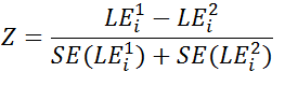
Figure 5: Healthy life expectancy at birth and age 65 using the GLF and APS, UK, 2009-11

Source: Office for national statistics
Download this image Figure 5: Healthy life expectancy at birth and age 65 using the GLF and APS, UK, 2009-11
.png (9.0 kB) .xls (28.2 kB)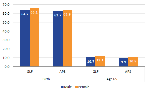
Figure 6: Disability-free life expectancy at birth and age 65 using the GLF and APS, UK, 2009-11
Source: Office for national statistics
Download this image Figure 6: Disability-free life expectancy at birth and age 65 using the GLF and APS, UK, 2009-11
.png (7.4 kB) .xls (28.2 kB)
Table 14: Table of differences between GLF and APS, years, UK, 2009 to 2011
| Measure | Age | Male | Female |
| HLE | Birth | 1.50 | 2.20 |
| Age 65 | 0.80 | 1.30 | |
| DfLE | Birth | 0.90 | 1.30 |
| Age 65 | 0.80 | 0.70 | |
| Source: Office for national statistics | |||
| Notes: | |||
| 1. Differences calculated on unrounded estimates | |||
Download this table Table 14: Table of differences between GLF and APS, years, UK, 2009 to 2011
.xls (27.1 kB)When comparing HLE and DfLE the GLF produces higher health expectancies estimates at birth and at age 65 for both genders. The difference in health state life expectancies is larger at birth than at age 65 and larger for females compared to males, apart from DfLE at age 65.
Effect on lower geographies
English regions and upper tier local authorities (UTLA) are already published using the APS. Previously they used the 16 to 19 health prevalence for all younger age groups and used an upper age group of 85 and over. The analysis will move to the same imputation method described in this paper and will also move to a 90 and over age group to be consistent with life expectancy calculations.
The following tables compare new method, which includes the new imputation and 90 and over final age group, to the published figures, which includes the old imputation method and an 85 and over final age group.
Table 15: HLE at birth, English Regions, 2010 to 2012
| 2010-12 - New methods | 2010-12 - Published | Difference | ||
| Male | North East | 59.7 | 59.5 | 0.2 |
| North West | 61.1 | 61.3 | -0.2 | |
| Yorkshire and The Humber | 60.9 | 61.2 | -0.3 | |
| East Midlands | 63.1 | 63.2 | -0.1 | |
| West Midlands | 62.1 | 62.3 | -0.3 | |
| East of England | 64.7 | 64.9 | -0.2 | |
| London | 63.1 | 63.2 | -0.2 | |
| South East | 65.5 | 65.8 | -0.4 | |
| South West | 65.1 | 65.2 | -0.1 | |
| Female | North East | 60.3 | 60.1 | 0.2 |
| North West | 61.8 | 61.8 | 0.0 | |
| Yorkshire and The Humber | 61.8 | 62.0 | -0.2 | |
| East Midlands | 63.5 | 63.6 | -0.1 | |
| West Midlands | 62.9 | 62.7 | 0.2 | |
| East of England | 66.1 | 66.1 | 0.0 | |
| London | 63.6 | 63.6 | 0.0 | |
| South East | 67.1 | 67.1 | 0.0 | |
| South West | 65.8 | 66.0 | -0.2 | |
| Source: Office for National Statistics | ||||
| Notes: | ||||
| 1. Differences calculated on unrounded estimates | ||||
Download this table Table 15: HLE at birth, English Regions, 2010 to 2012
.xls (28.2 kB)For healthy life expectancy at birth there are very small differences that are both positive and negative. The largest difference is for males in the South East, the smallest differences were less than 1 decimal place and occurred in a number of regions.
Table 16: DFLE at birth, English Regions, 2010 to 2012
| 2010-12 - New methods | 2010-12 - Published | Difference | ||
| Male | North East | 61.0 | 61.2 | -0.2 |
| North West | 61.3 | 61.7 | -0.4 | |
| Yorkshire and The Humber | 61.5 | 61.9 | -0.3 | |
| East Midlands | 62.9 | 63.2 | -0.3 | |
| West Midlands | 62.5 | 62.9 | -0.4 | |
| East of England | 64.5 | 64.9 | -0.3 | |
| London | 64.0 | 64.4 | -0.4 | |
| South East | 65.6 | 66.3 | -0.7 | |
| South West | 65.1 | 65.5 | -0.4 | |
| Female | North East | 60.2 | 60.4 | -0.2 |
| North West | 61.8 | 62.0 | -0.2 | |
| Yorkshire and The Humber | 61.8 | 62.2 | -0.4 | |
| East Midlands | 62.5 | 62.7 | -0.2 | |
| West Midlands | 62.8 | 63.1 | -0.3 | |
| East of England | 65.3 | 65.4 | -0.2 | |
| London | 64.0 | 64.5 | -0.5 | |
| South East | 66.4 | 66.8 | -0.5 | |
| South West | 65.4 | 65.9 | -0.5 | |
| Source: Office for National Statistics | ||||
| Notes: | ||||
| 1. Differences calculated on unrounded estimates | ||||
Download this table Table 16: DFLE at birth, English Regions, 2010 to 2012
.xls (28.2 kB)The differences for DfLE are slightly larger but are all still less than a year difference. There was a decrease in each region in regards to DfLE. The largest change can be seen for males in South East with a difference of 0.7 years.
The data for 2010 to 2012 published and 2010 to 2012 estimates with the census imputation and 90 and over age group at birth can be found in the attached spreadsheet. For HLE differences between methods across UTLAs range from minus 1.9 years to plus 2.6 years. For DfLE the differences were between minus 1.1 and plus 3.1. For both health state expectancies 90% of areas had differences less than 1 year. These comparisons though should be read in the context of moving to a 90 and over upper age group, which has a predominant effect of reducing the health expectancy estimate as with life expectancy reported earlier.
Back to table of contents6. New imputation method and impact on confidence intervals
National
The width of 95% confidence intervals around measures of health expectancy at birth and age 65 will be affected by the change to a 90 and over upper age band and the imputation based on the proportional difference in health state prevalence found at 2011 Census for those aged below 16 and above 84.
The sample design of the Annual Population Survey, from which the health state prevalence estimates are calculated, is systematic and stratified, not a simple random sample. This means standard errors of estimates need correction for the data collection design effect. The design effect is the ratio of the actual variance, under the sampling method used, to the variance computed under the assumption of simple random sampling. A design effect value of 2, means the sample variance is twice as big as it would be under a simple random sample.
For the latest published period, 2012-14, the new method of imputation and use of an upper age group of 90+ has produced a reduction in the variance and hence the confidence interval width of both Healthy Life Expectancy and Disability-free Life Expectancy and at age 65 at the UK and its constituent country level. As the move to closing the life table at 90+ caused an increase in the variance of life expectancy, the reduction observed for health expectancy is caused by the change in the imputation method which outweighs any effect brought about by closing the life table at 90+. The percentage change in the variance and the confidence interval width for each country and the UK is shown below.
Table 17 Variance and confidence interval width of healthy life expectancy at birth and at age 65 using different methods: UK and Constituent Countries, 2012 to 2014
| At Birth | Old Imputation Method and life table closed at 85+ | New Imputation Method and life table closed at 90+ | ||||||
| Country | Males | Females | Males | Females | ||||
| Variance | 95% CI width (years) | Variance | 95% CI width (years) | Variance | 95% CI width (years) | Variance | 95% CI width (years) | |
| United Kingdom | 0.0059 | 0.30 | 0.0070 | 0.33 | 0.0048 | 0.27 | 0.0053 | 0.29 |
| England | 0.0074 | 0.34 | 0.0089 | 0.37 | 0.0061 | 0.31 | 0.0068 | 0.32 |
| Scotland | 0.0459 | 0.84 | 0.0522 | 0.90 | 0.0377 | 0.76 | 0.0409 | 0.79 |
| Wales | 0.0502 | 0.88 | 0.0525 | 0.90 | 0.0402 | 0.79 | 0.0429 | 0.81 |
| Nothern Ireland | 0.2140 | 1.81 | 0.2254 | 1.86 | 0.1819 | 1.67 | 0.1862 | 1.69 |
| At age 65 | Old Imputation Method and life table closed at 85+ | New Imputation Method and life table closed at 90+ | ||||||
| Country | Males | Females | Males | Females | ||||
| Variance | 95% CI width (years) | Variance | 95% CI width (years) | Variance | 95% CI width (years) | Variance | 95% CI width (years) | |
| United Kingdom | 0.0039 | 0.25 | 0.0046 | 0.27 | 0.00301 | 0.21502 | 0.00325 | 0.22357 |
| England | 0.0049 | 0.27 | 0.0058 | 0.30 | 0.00377 | 0.24069 | 0.00412 | 0.25149 |
| Scotland | 0.0286 | 0.66 | 0.0317 | 0.70 | 0.0228 | 0.59189 | 0.0231 | 0.59584 |
| Wales | 0.0259 | 0.63 | 0.0294 | 0.67 | 0.0205 | 0.56124 | 0.02276 | 0.59145 |
| Nothern Ireland | 0.1397 | 1.47 | 0.1497 | 1.52 | 0.11656 | 1.33834 | 0.11181 | 1.3108 |
| Source: Annual Population Survey, Death Registrations, Mid-year population estimates, Census 2011 | ||||||||
Download this table Table 17 Variance and confidence interval width of healthy life expectancy at birth and at age 65 using different methods: UK and Constituent Countries, 2012 to 2014
.xls (29.2 kB)Subnational HLE: changes in variance and confidence interval width
The variance of HLE at birth contracted for all regions, but contracted the most for females in the East Midlands and least for males in the North West. The reduction in the variance caused the confidence interval width to contract across regions on average by 0.07 of a year.
At age 65 the variance in HLE contracted by 22.7% overall and fell in each region for each sex. The confidence interval width also fell on average by 0.1 of a year, with the largest fall in Yorkshire and the Humber for women where it narrowed by 0.14 of a year. Generally the fall in the confidence interval width was larger for women than men.
For HLE at birth, more than 90% of upper tier local authorities had a smaller variance closing the life table at 90 and over and using adjustment factors for prevalence imputation. On average the variance shrunk by 9.9%. The largest shrinkage occurred in Wokingham 27.3% for males and Luton (34.7%) for females, but there were also large shrinkages in Trafford, Camden, West Berkshire and Central Bedfordshire for males, and for females in Southwark, South Gloucestershire and Hackney. The largest increase in variance occurred in the London Borough of Lambeth where it increased by 26.6% for males and by 9.5% for females in Enfield. On average the confidence interval width shrunk by 0.16 of a year for males and 0.25 of a year for females. The largest shrinkage was 0.6 of a year in Camden and the largest expansion of 0.75 of a year in Lambeth for males. The largest shrinkage for females occurred in Southwark of 1.22 years and the largest increase was in Lambeth of 0.29 of a year.
The impact of changing the closure of the life table at 90 and over and changing the method of imputation has been to improve the precision for the majority of areas. The average confidence interval width using the new methods across upper tier local authorities was 3.72 years compared with 3.88 years using the old methods for males. For females it was 3.97 and 4.22 years respectively.
For HLE at age 65 the variance increased in 9 UTLAs for males and 3 for females and decreased in 141 UTLAs for males and 147 for females. The largest increase of 20.7% for males occurred in Lambeth, while the largest contraction for males of 52.3% occurred in Central Bedfordshire; for females the largest increase of 20.1% occurred in Enfield, and the largest reduction of 66.6%| occurred in Southwark. On average, the variance across UTLAs shrunk by 18.6% for males and by 22.7% for females. The confidence interval width narrowed on average by 0.31 of a year for males and 0.41 of a year for females.
The percentage change in the variance and the confidence interval width for each country and the UK is available in the accompanying reference tables published alongside this report. The pattern of variance and confidence interval width reduction was also observed for DFLE and we can provide these comparisons on request.
Back to table of contents7. Future work
We will be publishing 2013 to 2015 healthy life expectancy and disability-free life expectancy in November 2016. This publication will include the use of the census proportions for adjustments and the use of a 90 and over upper age group for regions and upper tier local authorities in England; in addition, health state life expectancies for the UK and constituent countries for the years 2009 to 2011 to 2013 to 2015 will also be included. Figures for English regions and UTLA will also be revised for the periods 2009 to 2011 to 2012 to 2014 using the new methods.
We are currently looking at ways to improve the health state life expectancies. We are currently investigating ways to combine the use of census data and survey data to obtain a more consistent picture of the transition in health state and disability-free prevalence over time across the UK.
Back to table of contents8. References
Australian Bureau of Statistics (2010) What is a Standard Error and Relative Standard Error? Reliability of estimates for Labour Force data.
Chiang CL (1979) Life table and mortality analysis. World Health Organisation
Jiaquan Xu MD, Kenneth D, Kochanek MA, Sherry L, Murphy BS, Betzaida Tejada-Vera, BS (2010) Deaths: Final data for 2007. Centre for Disease Control and Prevention, National Vital Statistics Reports; Vol 58, no 19
ONS (2013) Characteristics of Older People: What does the 2011 Census tell us about the "oldest old" living in England & Wales?
ONS (2015) National Life Tables for England and Wales
Silcocks PBS, Jenna DA, Reza R (2001) Life expectancy as a summary of mortality in a population: statistical considerations and suitability for use by health authorities. J Epidemiol Community Health 55:38-43
ONS (2013b) Update to the Methodology used to Calculate Health Expectancies
Back to table of contents