1. What is uncertainty?
Many of our statistics rely on data collected from surveys. We are often interested in the characteristics of the population of people or businesses as a whole, but usually survey a sample of the population rather than everyone. This is timelier and more cost-effective and, if the sample is large enough and well designed, can lead to accurate statistics.
Using a sample means that our statistics are usually accompanied by measures of uncertainty. Uncertainty relates to how the estimate might differ from the “true value” and these measures help users of ONS statistics to understand the degree of confidence in the outputs. These measures of uncertainty include:
standard error
confidence interval
coefficient of variation
statistical significance
Understanding sampling and the effect it has on statistics is also important for interpreting these measures of uncertainty.
Back to table of contents2. Sampling the population
Sampling involves selecting a subset of a population from which characteristics of the entire population can be estimated. Surveying a sample rather than an entire population is more-cost effective and allows data and findings to be published sooner.
Information is not gathered from the whole population, so results from sample surveys are estimates of the unknown population values. One sample is selected at random but other potential samples could have been selected, which may have produced different results.
The difference between a statistic derived from a sample and the population value is caused by what are known as sampling error and non-sampling errors.
Sampling error
Sampling error is caused by the use of a sample of the population, rather than the entire population. Estimates derived from a sample are likely to differ from the unknown population value because only a subset of the population have provided information. Designing a sample using a scientific approach can help to minimise sampling error and create estimates that are precise and unbiased.
The standard error, coefficient of variation and confidence interval can be used to help interpret the possible sampling error, which of course, is unknown. Standard errors are important for interpreting changes in the population estimates over time. A test of statistical significance could be used to decide whether the difference between estimates from different samples is caused by a real change in the population, or whether it is because of the effects of random sampling alone.
Non-sampling errors
Other sources of error are called non-sampling errors. These include:
businesses or individuals being unreachable
businesses or individuals refusing to respond
respondents giving inaccurate answers
processing or analysis errors
These errors would be present in the statistics even if the entire population had been surveyed. For example, inaccurate answers to a question about money spent on fuel would lead to a difference between the estimate and the population value even if the entire population were surveyed. These errors are usually very difficult to quantify and to do so would require additional and specific research.
Back to table of contents3. Standard error
The standard error is the simplest measure of how precise a survey-based estimate is.
The standard error can be used as a guide to help interpret the possible sampling error. It shows how close the estimate based on sample data might be to the value that would have been taken from the whole population. It is measured using the same units as the estimate itself and, in general, the closer the standard error is to zero, the more precise the estimate. Smaller values show a greater level of precision.
Standard errors are also based on sample data so are an unknown statistic, and are usually estimated themselves.
Example:
The non-financial business economy estimates are taken from the Annual Business Survey. The standard error for estimates of various industry sectors is used to assess how precise total turnover estimates are. The estimates for education, and water and waste management differ in size, as do their standard errors. However, the relative standard errors show they have similar levels of relative precision (Table 1).
| Total turnover in | Standard error in | Relative standard error (or coefficient of variation)² | |
|---|---|---|---|
| £ millions¹ | £ millions² | ||
| Industry 1: Education (private provision only) | 42,649 | 526.8 | 0.01 (or 1%) |
| Industry 2: Water supply; sewerage, waste management and remediation activities | 34,677 | 222.7 | 0.01 (or 1%) |
Download this table Table 1: Total turnover estimates, standard error and relative standard error for education and water and waste management, UK, 2016
.xls .csvNotes:
- Data are from Non-financial business economy, UK: Sections A to A 2017 revised results.
- Data are from Non-financial business economy, UK: quality measures 2017 revised results.
4. Coefficient of variation
The coefficient of variation makes it easier to understand whether a standard error is large compared with the estimate itself.
The coefficient of variation (CV) is used to compare the relative precision across surveys (or variables) and is usually shown as a percentage. It is a unitless quantity, and so allows us to compare estimates with different scales of measurement. It is also known as the relative standard error and is calculated by dividing the standard error of an estimate by the estimate itself.
Similar to the standard error, the closer the coefficient of variation is to zero, the more precise the estimate is. Where it is above 50%, the estimate is very unprecise and the confidence intervals around the estimate will effectively contain zero.
The coefficient of variation should not be used for estimates of values that are close to zero or for percentages.
Example:
The total turnover of plastering businesses in the UK was estimated at £2,322 million in 2016, with a standard error of £201 million. A different survey estimated that the total number of people employed full-time in agriculture, forestry and fishing in the UK was 155,000 in 2016, with a standard error of 12,400 employees
It is difficult to compare these two standard errors. By calculating the coefficient of variation for each, the results show that both estimates have a similar level of precision:
£201 million divided by £2,322 million equals 0.087 – a coefficient of variation of 8.7%
12,400 divided by 155,000 equals 0.08 – a coefficient of variation of 8%
The data for this example are from Non-financial business economy, UK: Sections A to S, Non-financial business economy, UK: quality measures, and Broad Industry Group (SIC) – Business Register and Employment Survey (BRED): Table 1.
Back to table of contents5. Confidence interval
Confidence intervals use the standard error to derive a range in which we think the true value is likely to lie.
A confidence interval gives an indication of the degree of uncertainty of an estimate and helps to decide how precise a sample estimate is. It specifies a range of values likely to contain the unknown population value. These values are defined by lower and upper limits.
The width of the interval depends on the precision of the estimate and the confidence level used. A greater standard error will result in a wider interval; the wider the interval, the less precise the estimate is.
Using a 95% confidence interval
A 95% confidence level is frequently used. This means that if we drew 20 random samples and calculated a 95% confidence interval for each sample using the data in that sample, we would expect that, on average, 19 out of the 20 (95%) resulting confidence intervals would contain the true population value and 1 in 20 (5%) would not. If we increased the confidence level to 99%, wider intervals would be obtained.
Example:
Estimates for July to September 2019 show 32.75 million people aged 16 years and over in employment in the UK, with a confidence interval of plus or minus 177,000 people based on the results from a sample. If we took a large number of samples repeatedly, 95% of the confidence intervals would contain the unknown population estimate.
The data for this example are from Labour market overview, UK: November 2019 and A11: Labour Force Survey sampling variability.
Calculating confidence intervals
To calculate confidence intervals around an estimate we use the standard error for that estimate. The estimate and its 95% confidence interval are presented as: the estimate plus or minus the margin of error.
The lower and upper 95% confidence limits are given by the sample estimate plus or minus 1.96 standard errors.
The margin of error is calculated as:
Margin of error = 1.96 × standard error
Example:
In 2016, the UK private education industry was estimated to have generated a total turnover of £42,649 million. The standard error for this estimate is £526.8 million.
The 95% confidence interval around this estimate is calculated as:
Margin of error = 1.96 × £526.8 million = £1,032.5 million
The 95% confidence interval is therefore £42,649 million plus or minus £1,032.5 million, which equals £41,616 million and £43,682 million respectively.
This means that if we drew 20 random samples and calculated an analogous confidence interval for each, on average, 19 out of 20 (95%) would contain the true population value and 1 in 20 (5%) would not. Therefore, there is a 95% chance that the true population value lies between £41,616 million and £43,682 million.
Data for this example come from Non-financial business economy, UK: Sections A to S 2017 revised results and Non-financial business economy, UK: quality measures 2017 revised results.
Back to table of contents6. Statistical significance
We can use statistical significance to decide whether we think a difference between two survey-based estimates reflects a true change in the population rather than being attributable to random variation in our sample selection.
Statistical significance helps us to establish what observed changes or relationships we should pay attention to, and which apparent changes may have occurred only as a result of randomness in the sampling.
A result is said to be statistically significant if it is likely not caused by chance or the variable nature of the samples. A defined threshold can help us test for change. If the test of statistical significance calculated from the estimates at different points in time is larger than the threshold, the change is said to be “statistically significant”.
A 5% standard is often used when testing for statistical significance. The observed change is statistically significant at the 5% level if there is less than a 1 in 20 chance of the observed change being calculated by chance if there is actually no underlying change.
Within the commentary of our statistical bulletins we will avoid using the term “significant” to describe trends in our statistics and will always use “statistically significant” to avoid any confusion for our users.
Example:
Estimates from the Annual Population Survey are based upon one of several samples that could have been drawn at that point in time. This means there is a degree of variability around the estimates. This can sometimes present misleading changes in figures because the people included in the sample are selected at random.
Figure 1: There has been a statistically significant decrease in the prevalence of smoking in the UK in 2018 compared with 2011
Proportion who were current smokers, all persons aged 18 years and over, UK, 2011 to 2018

Source: Office for National Statistics – Annual Population Survey
Download this image Figure 1: There has been a statistically significant decrease in the prevalence of smoking in the UK in 2018 compared with 2011
.png (15.8 kB) .xlsx (160.9 kB)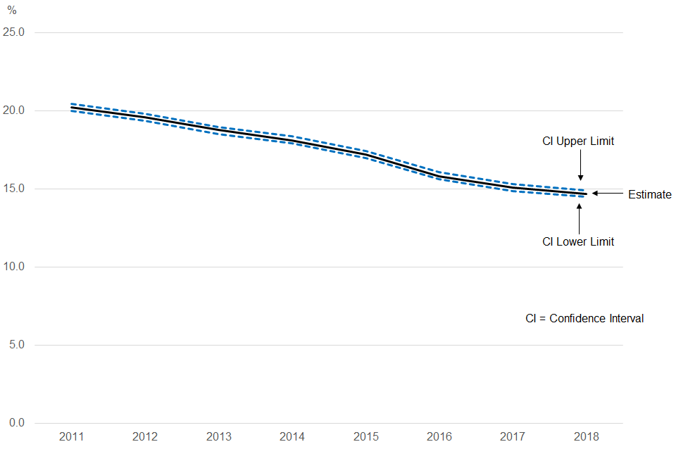
The proportion of people aged 18 years and over smoking cigarettes in the UK is estimated to have changed from 20.2% in 2011 to 14.7% in 2018. But we cannot assume that this change represents a real decrease in the prevalence of smoking. It could be the result of variations in the sample estimates, which make the differences between the estimates larger than the real change in smoking prevalence.
The test of statistical significance found that the difference between the estimates was larger than expected if it had only been caused by random sampling. This means that the difference is likely to reflect a true decrease in the prevalence of smoking in the UK between 2011 and 2018 rather than being attributable to random variation in our sample selection between these two years.
Back to table of contents