Access to details of the methodology and variables used for the 2011 area classifications covering local authority districts, health areas and Output Areas.
Local authority districts
Methodology note for the 2011 Area Classification for Local Authorities: version 2
Introduction
This section outlines the methodology used to produce the 2011 Area Classification for Local Authorities. The classification places each of the 391 UK local authority districts into different groups (clusters) based on their 2011 Census characteristics – using census results covering demographic, household, housing, socio-economic and employment topics, with similar local authorities grouped together. In this way, local authorities across the UK can be compared and classified according to these particular census characteristics.
2011 Area Classification for Local Authorities: version 2
As a result of a number of data and methodological issues that have come to light after publication of the 2011 Area Classification for Local Authorities in July 2015, a revised and corrected version (version 2) of the classification was published in July 2017.
This methodology note is unchanged in detail from the previously published methodology note in a pdf format. The original methodology note outlined the use of a K-means technique to produce the hierarchical classification. In fact, with the previously published version of the classification, a K-median clustering technique was unintentionally used, rather than K-means as intended. The previously published methodology note was therefore incorrect in this respect.
Choice of statistics
The analysis was carried out using the 2011 Census Key Statistics and Quick Statistics tables, as published by Office for National Statistics (ONS) for England and Wales, National Records of Scotland (NRS) for Scotland, and the Northern Ireland Statistics and Research Agency (NISRA) for Northern Ireland. Only census statistics that were consistent1 across the whole of the UK were considered for the classification.
An initial 167 socio-economic and demographic census statistics, and derived statistics, covered the main dimensions of the census. For presentation purposes, these have been defined within five different domains:
- demographic structure
- household composition
- housing
- socio-economic character
- employment
Strongly correlated statistics were removed to avoid the duplication of particular factors. This allowed the minimum number of statistics to be included so that the main census domains were represented using the available data.
Notes:
- Two exceptions – firstly, questions relating to main language, where the questions asked by country were slightly different, though the information gathered broadly comparable, and secondly, in Scotland, unlike England, Wales and Northern Ireland, full-time students who were working did not have method of travel to work reported in the published tables originally used – as this was assumed to relate to place of study instead.
Data preparation
Before any analysis of the initial 167 statistics of the local authority data could be done, the data needed to be prepared to assist with the processes used in the selection of the final statistics. For the data preparation, for the majority of the census statistics used, figures were converted to raw percentages. A few statistics, such as those relating to area and population density, could not be converted into percentages and were left unchanged.
Data transformation
The dataset created from the data preparation stage was investigated to examine the extent to which outliers may exist within the data and the data ranges. As a result of this investigation, three different transformation techniques were tested, tried and considered to reduce skew in the dataset:
- log
- box-cox
- inverse hyperbolic sine
These three techniques all perform a “normalisation” function. The impact of these three data transformation techniques was later tested with the final assignment of areas into categories after “clustering”.
By transforming the data to a log (logarithmic) scale, the problem of very high value outliers is greatly reduced as the differences between values at the extremities of the dataset are reduced by more than the differences between the smaller average values. The box-cox method is considered better than the log method for dealing with different distributions that may occur between statistics, whilst the inverse hyperbolic sine method is considered better at dealing with datasets with a large number of zero values.
Data standardisation
All clustering techniques are based on the similarity or dissimilarity of the cases to be clustered. This is measured by constructing a distance matrix reflecting all the variables in the dataset for each case. It is clear that problems will occur if there are differing scales or magnitudes among the variables. In general, statistics with larger values and greater variation will have more impact on the final similarity measure. It is necessary to ensure each statistic is equally represented in the distance measure by standardising the data.
Two methods of standardisation were considered:
- range standardisation
- inter-decile range standardisation
The range standardisation method compares each value of a variable, Xi, to the minimum value Xmin. This is then divided by the distance between the minimum value, Xmin, and the maximum value, Xmax, of the variable. After the data have been range standardised, each variable has a range of one with the maximum value being one and minimum value being zero. This method does not work well if the data contain extreme outliers. Range standardisation has been used with a number of ONS area classifications covering other different geographies.
The inter-decile range standardisation method is a variation of the range standardisation method that overcomes the problems associated with outliers. It compares each value of a variable, Xi, to the median, which is then divided by the distance between the 90th percentile and the 10th percentile. This standardisation method was used with the 2001 Area Classification for Local Authorities.
Final selection of statistics
The process of reducing the 167 initial statistics to a list of final statistics is to cluster required multiple steps with the overall aim of reducing the number of statistics so that the remaining ones were the most important for the classification. By applying different combinations of data transformation and data standardisation techniques, six unique datasets (three multiplied by two) were created and evaluated.
From this evaluation, a list of 59 final statistics were chosen (see Variables section) and the data preparation, data transformation and data standardisation techniques were repeated to produce a further six datasets; all with the potential to be used for cluster analysis for the production of the final classification.
These six datasets were then evaluated as part of a clustering suitability assessment.
Clustering is a technique for finding similarity groups in data, called clusters. For the purpose of the local authority classification, this technique attempts to group local authorities together by similarity alone.
The K-means algorithm clusters data by trying to separate samples (local authorities) in n groups of equal variance, minimising a criterion known as the inertia or within-cluster sum-of-squares. This algorithm requires the number of clusters (that is, supergroups, groups and subgroups) to be specified and is an iterative process.
A standard K-means clustering technique was applied to group together local authorities with similar characteristics; this approach was consistent with the clustering technique used for the previous 2001 Area Classification for Local Authorities.
Identifying an optimum dataset and number of clusters
Of the six datasets from different combinations of data transformation and data standardisation methods, a series of checks were undertaken to identify the “best” dataset for clustering using the 59 final statistics. This included checking for:
- datasets that had skewness values above one or less than negative one
- datasets that led to the creation of very small clusters, accounting for a small percentage of the population
- datasets that led to the creation of different clusters that were not considered sufficiently distinguishable
These three checks were considered to help identify an optimum dataset and to reject the other datasets.
Creating a hierarchical classification using K-means
When the K-means algorithm is run on the dataset n clusters are produced. The original dataset is then split into n separate datasets (representing the highest level of the hierarchy). Each of the new datasets then has the K-means algorithm run on them separately to create the second level of the hierarchy. The second level of the hierarchy is then separated into m separate datasets and each one has the K-means algorithm run on them to create the lowest level of the hierarchy.
With the six datasets to be evaluated, a different number of cluster permutations were tested using K-means, based on a preferred range of five to nine clusters for the supergroup level, reflecting a similar hierarchical structure to the 2001 Area Classification for Local Authorities. A final decision made on both the dataset and cluster numbers used to create the final 2011 Area Classification for Local Authorities was based on qualitative and quantitative assessments, and subjective judgement.
The preferred dataset was created using the following combination of data transformation and data standardisation methods:
- data transformation – inverse hyperbolic sine (method 3)
- data standardisation – inter-decile range standardisation (method 2)
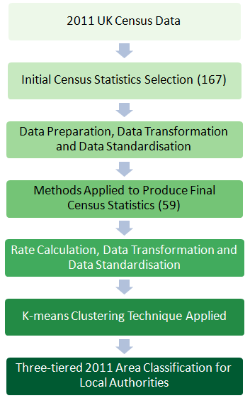
The resultant three-tier classification contains 8 supergroups, 16 groups and 24 subgroups. Finally, in addition to allocated codes for each cluster of the 2011 Area Classification for Local Authorities, names were also created to aid the understanding of a cluster’s characteristics.
Methodology overview: local authorities
Figure 1 provides an overview of the methodology used to produce the 2011 Area Classification for Local Authorities.
Variables used to create the 2011 Area Classification for Local Authorities
Introduction
This section lists the 59 2011 Census statistics and statistics variables that were used to create the 2011 Area Classification for Local Authorities, together with a glossary of some of the definitions used.
Glossary
Old EU countries – refers to the 15 pre-2004 accession countries: Austria, Belgium, Denmark, Finland, France, Germany, Greece, Irish Republic, Italy, Luxembourg, Netherlands, Portugal, Spain, Sweden and the UK.
New EU countries – refers to the 10 accession countries who joined the EU in 2004: Cyprus, Czech Republic, Estonia, Hungary, Latvia, Lithuania, Malta, Poland, Slovakia and Slovenia, and the two countries who joined in 2007 – Bulgaria and Romania.
Industries – based on aggregations of industries from the Standard Industrial Classification 2007 (SIC 2007), including:
- agriculture, forestry and fishing
- mining, quarrying or construction industries
- manufacturing industry
- energy, water or air conditioning supply industries
- wholesale and retail trade; repair of motor vehicles and motor cycles industries
- transport or storage industries
- accommodation or food service activities industries
- information and communication or professional, scientific and technical activities industries
- financial, insurance or real estate industries
- administrative or support service activities industries
- public administration or defence; compulsory social security industries
Qualifications – refers to different past and present qualifications, including:
- level 1, examples include GCSEs (grades D to G) and diplomas (City and Guilds, BTEC)
- level 2, examples include GCSEs (grades A* to C) and O Levels (grades A to C)
- level 3, examples include A Levels (grades A to E) and AS Levels
- level 4 and above, examples include Higher National Certificates (HNCs) and degrees
For more information, please contact us via email at areaclassifications@ons.gov.uk
Table 1: List of 59 final 2011 Census statistics
| Number | Description | Domain |
|---|---|---|
| 1 | Percentage of persons living in a communal establishment | Demographic structure |
| 2 | Number of persons per hectare | |
| 3 | Percentage of persons aged 0 to 4 years | |
| 4 | Percentage of persons aged 5 to 14 years | |
| 5 | Percentage of persons aged 25 to 44 years | |
| 6 | Percentage of persons aged 45 to 64 years | |
| 7 | Percentage of persons aged 65 to 89 years | |
| 8 | Percentage of persons aged 90 years and over | |
| 9 | Percentage of persons aged 16 years and over who are single | |
| 10 | Percentage of persons aged 16 years and over who are married or in a registered same-sex civil partnership | |
| 11 | Percentage of persons aged 16 years and over who are divorced or separated | |
| 12 | Percentage of persons who are white | |
| 13 | Percentage of persons who have mixed ethnicity or are from multiple ethnic groups | |
| 14 | Percentage of persons who are Asian/Asian British: Indian/Pakistani/Bangladeshi | |
| 15 | Percentage of persons who are Asian/Asian British: Chinese and Other | |
| 16 | Percentage of persons who are Black/African/Caribbean/Black British | |
| 17 | Percentage of persons who are Arab or are from another ethnic group | |
| 18 | Percentage of persons whose country of birth is the UK or Ireland | |
| 19 | Percentage of persons whose country of birth is in the old EU (pre 2004 accession countries) | |
| 20 | Percentage of persons whose country of birth is in the new EU (post 2004 accession countries) | |
| 21 | Percentage of persons whose main language is not English and cannot speak English well or at all1 | |
| 22 | Percentage of households with no children | House-hold composition |
| 23 | Percentage of households with non-dependent children | |
| 24 | Percentage of households with full-time students | |
| 25 | Percentage of households who live in a detached house or bungalow | Housing |
| 26 | Percentage of households who live in a semi-detached house or bungalow | |
| 27 | Percentage of households who live in a terrace or end-terrace house | |
| 28 | Percentage of households who live in a flat | |
| 29 | Percentage of households who live in a caravan or other mobile or temporary structure | |
| 30 | Percentage of households who own or have shared ownership of property | |
| 31 | Percentage of households who are social renting | |
| 32 | Percentage of households who are private renting | |
| 33 | Percentage of households who have one fewer room or less rooms than required | |
| 34 | Individuals day-to-day activities limited a lot or a little (Standardised Illness Ratio) | Socio-Economic |
| 35 | Percentage of persons providing unpaid care | |
| 36 | Percentage of persons aged 16 years and over whose highest level of qualification is Level 1, Level 2 or Apprenticeship | |
| 37 | Percentage of persons aged 16 years and over whose highest level of qualification is Level 3 qualifications | |
| 38 | Percentage of persons aged 16 years and over whose highest level of qualification is Level 4 qualifications and above | |
| 39 | Percentage of persons aged 16 years and over who are schoolchildren or full-time students | |
| 40 | Percentage of households with 2 or more cars or vans | |
| 41 | Percentage of persons aged between 16 and 74 years who use public transport to get to work | |
| 42 | Percentage of persons aged between 16 and 74 years who use private transport to get to work | |
| 43 | Percentage of persons aged between 16 and 74 years who walk, cycle or use an alternative method to get to work | |
| 44 | Percentage of persons aged between 16 and 74 years who are unemployed | Employment |
| 45 | Percentage of employed persons aged between 16 and 74 years who work part time | |
| 46 | Percentage of employed persons aged between 16 and 74 years who work full-time | |
| 47 | Percentage of employed persons aged between 16 and 74 years who work in the agriculture, forestry or fishing industries | |
| 48 | Percentage of employed persons aged between 16 and 74 years who work in the mining, quarrying or construction industries | |
| 49 | Percentage of employed persons aged between 16 and 74 years who work in the manufacturing industry | |
| 50 | Percentage of employed persons aged between 16 and 74 years who work in the energy, water or air conditioning supply industries | |
| 51 | Percentage of employed persons aged between 16 and 74 years who work in the wholesale and retail trade; repair of motor vehicles and motor cycles | |
| 52 | Percentage of employed persons aged between 16 and 74 years who work in the transport or storage industries | |
| 53 | Percentage of employed persons aged between 16 and 74 years who work in the accommodation or food service activities industries | |
| 54 | Percentage of employed persons aged between 16 and 74 years who work in the information and communication or professional, scientific and technical activities | |
| 55 | Percentage of employed persons aged between 16 and 74 years who work in the financial, insurance or real estate activities | |
| 56 | Percentage of employed persons aged between 16 and 74 years who work in the administrative or support service activities industries | |
| 57 | Percentage of employed persons aged between 16 and 74 years who work in the public administration or defence; compulsory social security industries | |
| 58 | Percentage of employed persons aged between 16 and 74 years who work in the education sector | |
| 59 | Percentage of employed persons aged between 16 and 74 years who work in the human health and social work activities industries | |
| Notes: | ||
| 1. This description relates to the 2011 Census question asked in England and Northern Ireland only (which applies just to residents aged three and over). | ||
Download this table Table 1: List of 59 final 2011 Census statistics
.xls (44.0 kB)For Wales and Scotland, the language question asked in the 2011 Census differed, so this statistic should be interpreted as follows (which also applies just to residents aged 3 years and over):
Wales – percentage of persons whose main language is not English or Welsh and they cannot speak English well or at all
Scotland – percentage of persons who cannot speak English well or at all, regardless of main language
Health areas
Methodology note for the 2011 Area Classification for Health Areas
Introduction
This section outlines the methodology used to produce the 2011 Area Classification for Health Areas. The classification places each of the 235 health areas in the UK into different groups (clusters) based on their 2011 Census characteristics with similar health areas grouped together – using census results covering demographic structure, household composition, housing, socio-economic character, and employment topics. In this way, health areas across the UK can be compared and classified according to their underlying census characteristics. The health areas used in the classification are clinical commissioning groups (CCGs) in England, local health boards in Wales, health boards in Scotland and health and social care boards in Northern Ireland.
Choice of statistics
The analysis was carried out using the 2011 Census Key Statistics and Quick Statistics tables, as published by Office for National Statistics (ONS) for England and Wales, National Records of Scotland (NRS) for Scotland, and the Northern Ireland Statistics and Research Agency (NISRA) for Northern Ireland. Only census statistics that were consistent1 across the whole of the UK were considered for the classification.
The census statistics used for the health area classification – 59 statistics (covering five different topics), were the same as those used for the local authority classification. For the health area classification, health areas were assigned to clusters based on the 24 subgroups with the local authority classification. In this way, the health area classification was not therefore created independently, but rather health areas were aligned instead to their “closest” local authority subgroup cluster (based on squared Euclidean distance measures), from which a group and supergroup allocation could then be identified.
There are 79 out of 235 UK health areas whose boundaries exactly align with local authority boundaries. Where this occurs the majority of health areas have been allocated to the same clusters as assigned in the local authority classification. However, there are four health areas that align with local authorities where these allocations differ (NHS Ashford CCG and Ashford, NHS North Somerset CCG and North Somerset, Shetland and Shetland Islands, and NHS Wiltshire CCG and Wiltshire).
These four health areas were assigned to different clusters than the local authorities covering the same areas because the methodology produces a cluster allocation that does not guarantee consistent (optimal) results for both the local authority and/or the health area classification.
Notes:
- Two exceptions – firstly, questions relating to main language, where the questions asked by country were slightly different, though the information gathered broadly comparable, and secondly, in Scotland, unlike England, Wales and Northern Ireland, full-time students who were working did not have method of travel to work reported in the published tables originally used – as this was assumed to relate to place of study instead.
Data preparation
With the data preparation, census statistics for health areas were acquired. The majority of these census statistics were estimates, and in such cases, these census estimates were converted to raw percentages. A couple of the statistics, relating to population density and the standardised illness ratio, were not suitable to be converted into percentages and were left unchanged.
Data transformation and standardisation
To reduce the skew in the dataset created from the data preparation stage, an inverse hyperbolic sine data transformation was applied, as was used for the local authority classification. This data transformation technique had previously been chosen for the local authority classification as this method was considered better at dealing with datasets with a large number of zero values, though other data transformation methods had also been considered.
All clustering techniques are based on the similarity or dissimilarity of the cases to be clustered. This is measured by constructing a distance matrix reflecting all the variables in the dataset for each case. It is clear that problems will occur if there are differing scales or magnitudes among the variables. In general, statistics with larger values and greater variation will have more impact on the final similarity measure. It is necessary to ensure each statistic is equally represented in the distance measure by standardising the data. To do this, the inter-decile range standardisation method was used, which is the same method as used for the 2011 Area Classification for Local Authorities, which is considered the best method at overcoming problems associated with outliers.
The inter-decile range standardisation is the same standardisation method as used for the local authority classification, upon which the health area classification is based. The denominator in the standardisation formula was the same as that used in the local authority classification so that the census statistics were on the same scale as the classification it was being assigned to.
The standardisation method compared each health area’s value, Xi, for each census statistic after transformation to the UK median for local authorities, XLA–med , and is then divided by the distance between the 90th percentile, XLA–90th, and the 10th percentile, XLA–10th.
The formula for calculating this is as follows:
The method measures the deviation from the local authority median and this makes the health area data more consistent with the local authority classification.
Distance measure
Once each of the 59 census statistics had been appropriately standardised, it was necessary to determine how “close” the census statistics were for the health areas, or how far apart they were. Most methods of cluster analysis begin with a matrix reflecting a quantitative measure of similarity for each health area. This is more commonly referred to as a similarity, distance, dissimilarity or proximity matrix. Two health areas may be considered “close” when their dissimilarity or distance is small or their similarity is large. There are many different measures that can be used to quantify proximity, with the Euclidean distance and the squared Euclidean distance (SED) being two of the most common. The SED was the chosen measure of similarity.
Two health areas X and Y are considered similar if the “distance” between them, based on census characteristics, is small. It used the following formula:
where Xi = value of variable i for health area X and Yi = value of variable i for health area Y
The distance between the two health areas is calculated as the sum of the squared differences between their values for each census statistic used.
Assignment to clusters
The health area classification was produced by assigning each health area to the “closest” one of the 24 local authority subgroups. This was defined as the subgroup whose centroid had the smallest Euclidean distance from the health area. When this was done, and health areas were initially assigned to local authority subgroups, the number of health areas (235 in total) assigned to each of the 24 local authority classification subgroups (based on 391 local authorities) was examined.
For the local authority subgroup, 3a1r Older Farming Communities, only two health areas were assigned, and for the subgroup 7c1r Prosperous Semi-Rural, there was just a single health area assigned. Rather than having health area subgroups with a very small number of assigned health areas, as had been initially identified, the group cluster was used to define these subgroups instead.
Other subgroups within the 3a English and Welsh Countryside group and 7c Town Living group were similarly reassigned for their subgroup allocation to the parent group cluster. As a result, there are 22 subgroups for the health area classification, compared with 24 for the local authority classification, and duplication of names for these two groups and subgroups.
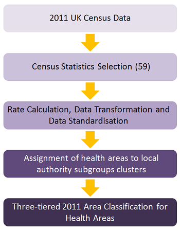
Methodology overview: health areas
Figure 2 provides an overview of the methodology used to produce the 2011 Area Classification for Health Areas.

Census statistics used to create the 2011 Area Classification for Health Areas
The same census statistics were used for creating the health area classification as were used for the local authority classification (but at health area level, rather than local authority level). Information about the census statistics used can be found under the section “Variables used to create the 2011 Area Classification for Local Authorities”.
Super Output Areas
Methodology note for the 2011 Area Classification for Super Output Areas
Introduction
This section outlines the methodology used to produce the 2011 Area Classification for Super Output Areas. The classification places each of the 42,619 Super Output Areas in the UK – comprising Lower Layer Super Output Areas in England and Wales, Data Zones in Scotland, and Super Output Areas in Northern Ireland, into different groups (clusters) based on their 2011 Census characteristics – using census results covering demographic, household, housing, socio-economic and employment topics, with similar Super Output Areas grouped together. In this way, Super Output Areas across the UK can be compared and classified according to their census-recorded characteristics.
Choice of statistics
The analysis was carried out using the 2011 Census Key Statistics and Quick Statistics tables, as published by Office for National Statistics (ONS) for England and Wales, National Records of Scotland (NRS) for Scotland, and the Northern Ireland Statistics and Research Agency (NISRA) for Northern Ireland. Only census statistics that were consistent1 across the whole of the UK were considered for the classification.
The same 60 census variables were chosen for use in this classification as were used for the output area classification. All the previous classifications published following the 2011 Census used almost consistent variables; considerable time and resource was therefore saved by continuing with the same variables as used for the output area classification rather than repeating previous work to test a much larger number of variables for suitability, initially before the selection of a final set of variables for producing the classification. The 60 variables chosen for the classification can be categorised into five different domains:
- demographic structure
- household composition
- housing
- socio-economic character
- employment
Notes:
Three exceptions:
- questions relating to main language, where the questions asked by country were slightly different, though the information gathered was broadly comparable
- in Scotland, unlike England, Wales and Northern Ireland, full-time students who were working did not have method of travel to work reported in the published tables originally used – as this was assumed to relate to place of study instead
- in Scotland, the question relating to educational attainment does not have an option to select for apprenticeships, unlike in England, Wales and Northern Ireland
Data preparation
For the data preparation, for the majority of the census statistics used, figures were converted to raw percentages. A few statistics, such as those relating to area and population density, could not be converted into percentages and were left unchanged.
Data transformation
The dataset created from the data preparation stage needed to be transformed to reduce the extent to which outliers existed within the data and the data ranges, thereby reducing the skewness in the dataset. The same transformation techniques were used as for the output area classification – inverse hyperbolic sine.
Data standardisation
All clustering techniques are based on the similarity or dissimilarity of the cases to be clustered. This is measured by constructing a distance matrix reflecting all the variables in the dataset for each case. Problems will occur if there are differing scales or magnitudes among the variables. In general, statistics with larger values and greater variation will have more impact on the final similarity measure. It is necessary to ensure each statistic is equally represented in the distance measure by standardising the data.
The same standardisation was chosen as for the output area classification – range standardisation.
The range standardisation method compares each value of a variable, Xi, to the minimum value Xmin. This is then divided by the distance between the minimum value, Xmin, and the maximum value, Xmax, of the variable. After the data have been range-standardised, each variable has a value between zero being the minimum value and one being the maximum value.
Clustering
Clustering is a technique for finding similarity groups in data, called clusters. For this classification, the clustering technique attempts to group Super Output Areas together by similarity alone.
The K-means algorithm clusters data by trying to separate samples of Super Output Areas in n groups of equal variance, minimising a criterion known as the inertia or within-cluster sum-of-squares. This algorithm requires the number of clusters initially for supergroups to be specified and is an iterative process, and then the number of groups within these supergroups to be specified.
A standard K-means clustering technique was applied to group together Super Output Areas with similar characteristics; this approach was consistent with the clustering technique used for other 2011 Census-based classifications. When the K-means algorithm is run on the dataset n clusters are produced. The original dataset is then split into n separate datasets (representing the highest level of the hierarchy – supergroups). Each of the new datasets then has the K-means algorithm run on them separately to create the second level of the hierarchy – groups.
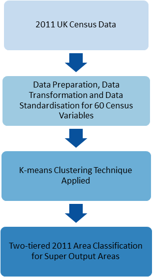
The resultant two-tier classification contains eight supergroups and 24 subgroups. Finally, in addition to allocated codes for each cluster of the 2011 Area Classification for Super Output Areas, names were also created to aid the understanding of a cluster’s characteristics.
Methodology overview
Figure 3 provides an overview of the methodology used to produce the 2011 Area Classification for Super Output Areas.
Variables used to create the 2011 Area Classification for Super Output Areas
Introduction
This section lists the 60 2011 Census statistics and statistics variables that were used to create the 2011 Area Classification for Super Output Areas, together with a glossary of some of the definitions used.
Glossary
Old EU countries – refers to the 15 pre-2004 accession countries: Austria, Belgium, Denmark, Finland, France, Germany, Greece, Irish Republic, Italy, Luxembourg, Netherlands, Portugal, Spain, Sweden and the UK.
New EU countries – refers to the 10 accession countries who joined the EU in 2004: Cyprus, Czech Republic, Estonia, Hungary, Latvia, Lithuania, Malta, Poland, Slovakia and Slovenia, and the two countries who joined in 2007 – Bulgaria and Romania.
Industries – based on aggregations of industries from the Standard Industrial Classification 2007 (SIC 2007), including:
- agriculture, forestry and fishing
- mining, quarrying or construction industries
- manufacturing industry
- energy, water or air conditioning supply industries
- wholesale and retail trade; repair of motor vehicles and motor cycles industries
- transport or storage industries
- accommodation or food service activities industries
- information and communication or professional, scientific and technical activities industries
- financial, insurance or real estate industries
- administrative or support service activities industries
- public administration or defence; compulsory social security industries
- education sector
- human health and social work activities industries
Qualifications – refers to different past and present qualifications, including:
- level 1, examples include GCSEs (grades D to G) and diplomas (City and Guilds, BTEC)
- level 2, examples include GCSEs (grades A* to C) and O Levels (grades A to C)
- level 3, examples include A Levels (grades A to E) and AS Levels
- level 4 and above, examples include Higher National Certificates (HNCs) and degrees
For more information, please contact us via email at areaclassifications@ons.gov.uk.
List of 60 final 2011 Census statistics
Table 2: List of 60 final 2011 Census statistics
| Number | Description | Domain |
|---|---|---|
| 1 | Percentage of persons living in a communal establishment | Demographic structure |
| 2 | Number of persons per hectare | |
| 3 | Percentage of persons aged 0 to 4 years | |
| 4 | Percentage of persons aged 5 to 14 years | |
| 5 | Percentage of persons aged 25 to 44 years | |
| 6 | Percentage of persons aged 45 to 64 years | |
| 7 | Percentage of persons aged 65 to 89 years | |
| 8 | Percentage of persons aged 90 years and over | |
| 9 | Percentage of persons aged 16 years and over who are single | |
| 10 | Percentage of persons aged 16 years and over who are married or in a registered same-sex civil partnership | |
| 11 | Percentage of persons aged 16 years and over who are divorced or separated | |
| 12 | Percentage of persons who are white | |
| 13 | Percentage of persons who have mixed ethnicity or are from multiple ethnic groups | |
| 14 | Percentage of persons who are Asian/Asian British: Indian | |
| 15 | Percentage of persons who are Asian/Asian British: Pakistani | |
| 16 | Percentage of persons who are Asian/Asian British: Bangladeshi | |
| 17 | Percentage of persons who are Asian/Asian British: Chinese and Other | |
| 18 | Percentage of persons who are Black/African/Caribbean/Black British | |
| 19 | Percentage of persons who are Arab or are from another ethnic group | |
| 20 | Percentage of persons whose country of birth is the UK or Ireland | |
| 21 | Percentage of persons whose country of birth is in the old EU (pre 2004 accession countries) | |
| 22 | Percentage of persons whose country of birth is in the new EU (post 2004 accession countries) | |
| 23 | Percentage of persons whose main language is not English and cannot speak English well or at all1 | |
| 24 | Percentage of households with no children | House-hold composition |
| 25 | Percentage of households with non-dependent children | |
| 26 | Percentage of households with full-time students | |
| 27 | Percentage of households who live in a detached house or bungalow | Housing |
| 28 | Percentage of households who live in a semi-detached house or bungalow | |
| 29 | Percentage of households who live in a terrace or end-terrace house | |
| 30 | Percentage of households who live in a flat | |
| 31 | Percentage of households who own or have shared ownership of property | |
| 32 | Percentage of households who are private renting | |
| 33 | Percentage of households who are social renting | |
| 34 | Percentage of households who have one fewer room or less rooms than required | |
| 35 | Individuals day-to-day activities limited a lot or a little (Standardised Illness Ratio) | Socio-Economic |
| 36 | Percentage of persons providing unpaid care | |
| 37 | Percentage of persons aged 16 years and over whose highest level of qualification is Level 1, Level 2 or Apprenticeship | |
| 38 | Percentage of persons aged 16 years and over whose highest level of qualification is Level 3 qualifications | |
| 39 | Percentage of persons aged 16 years and over whose highest level of qualification is Level 4 qualifications and above | |
| 40 | Percentage of persons aged 16 years and over who are schoolchildren or full-time students | |
| 41 | Percentage of households with 2 or more cars or vans | |
| 42 | Percentage of persons aged between 16 and 74 years who use public transport to get to work | |
| 43 | Percentage of persons aged between 16 and 74 years who use private transport to get to work | |
| 44 | Percentage of persons aged between 16 and 74 years who walk, cycle or use an alternative method to get to work | |
| 45 | Percentage of persons aged between 16 and 74 years who are unemployed | Employment |
| 46 | Percentage of employed persons aged between 16 and 74 years who work part time | |
| 47 | Percentage of employed persons aged between 16 and 74 years who work full-time | |
| 48 | Percentage of employed persons aged between 16 and 74 years who work in the agriculture, forestry or fishing industries | |
| 49 | Percentage of employed persons aged between 16 and 74 years who work in the mining, quarrying or construction industries | |
| 50 | Percentage of employed persons aged between 16 and 74 years who work in the manufacturing industry | |
| 51 | Percentage of employed persons aged between 16 and 74 years who work in the energy, water or air conditioning supply industries | |
| 52 | Percentage of employed persons aged between 16 and 74 years who work in the wholesale and retail trade; repair of motor vehicles and motor cycles | |
| 53 | Percentage of employed persons aged between 16 and 74 years who work in the transport or storage industries | |
| 54 | Percentage of employed persons aged between 16 and 74 years who work in the accommodation or food service activities industries | |
| 55 | Percentage of employed persons aged between 16 and 74 years who work in the information and communication or professional, scientific and technical activities | |
| 56 | Percentage of employed persons aged between 16 and 74 years who work in the financial, insurance or real estate activities | |
| 57 | Percentage of employed persons aged between 16 and 74 years who work in the administrative or support service activities industries | |
| 58 | Percentage of employed persons aged between 16 and 74 years who work in the public administration or defence; compulsory social security industries | |
| 59 | Percentage of employed persons aged between 16 and 74 years who work in the education sector | |
| 60 | Percentage of employed persons aged between 16 and 74 years who work in the human health and social work activities industries | |
| Notes: | ||
| 1. This description relates to the 2011 Census question asked in England and Northern Ireland only (which applies just to residents aged three and over). | ||
Download this table Table 2: List of 60 final 2011 Census statistics
.xls (44.5 kB)For Wales and Scotland, the language question asked in the 2011 Census differed, so this statistic should be interpreted as follows (which also applies just to residents aged 3 years and over):
- Wales – percentage of persons whose main language is not English or Welsh and they cannot speak English well or at all
- Scotland – percentage of persons who cannot speak English well or at all, regardless of main language
Output Areas
Methodology information for the 2011 Area Classification for Output Areas
Information detailing the methodology and variables in creating the 2011 Area Classification for Output Areas is available:
- Methodology note for the 2011 Area Classification for Output Areas (PDF, 392KB)
- 2011 output area classification variables (PDF, 111KB)
Update 15 April 2015
An error was found in the labelling of two census variables (numbered 32 and 33 in the supporting documentation) used in helping to define two subgroups. As a result two subgroups have now been renamed:
- 4a1 is now Social Renting Young Families (previously Private Renting Young Families)
- 4a2 is now Private Renting New Arrivals (previously Social Renting New Arrivals)
All supporting material has been updated to reflect these changes, in particular this affects references to households privately renting and socially renting in the pen portraits.
We apologise for any inconvenience caused.