Table of contents
- Introduction
- Column A fact sheet
- Column B, Part A, fact sheet
- Column B, Part B, fact sheet
- Column E fact sheet
- Column G fact sheet
- Column H fact sheet
- Column K fact sheet
- Column H: Detailed methodology (introduction)
- Column H: Overview of the models
- Column H: The new State Pension model
- Column H: Changes affecting both models
- Column H: Using the model outputs to produce Column H
1. Introduction
This methodology article presents a fact sheet for each column in Table 29: Accrued-to-date pension entitlements in social insurance for the UK for accounting year 2015. The layout of the fact sheets is established by Eurostat; all European Union member states have been asked to complete them for 2015. The fact sheets are presented in Sections 2 to 8.
There are no fact sheets for columns which are not applicable in the UK because the type of pension scheme does not exist (Columns D and F); or for Columns C and I, which are the sum of other columns (sub-total and total respectively); or for Column J, which is the result of subtracting Column K from Column I.
In addition, for Column H (social security pensions), this article provides further detail on the models used to produce the estimates (Sections 9 to 12). Finally, in Section 13, it explains how the model outputs feed into each row of Column H.
Back to table of contents2. Column A fact sheet
General description of the scheme and the calculation model
Coverage of the scheme
Column A comprises defined contribution (DC) pensions for (mainly) private sector employees. The Annual Survey of Hours and Earnings 2016 estimates that in 2015, 46% of private sector employees contributed to a workplace DC pension scheme. Column A also includes some public sector employee pensions provided by insurers, which are not separately identifiable.
The UK has thousands of DC pension schemes, both occupational (trust-based) and personal (contract-based). DC occupational pension schemes include the multi-employer “master trusts” set up since 2012 to provide pensions under the auto-enrolment programme where the employer does not already have a workplace pension scheme. Personal pensions are mainly provided by insurance companies and may be “group” personal pensions (within scope of Table 29) or “individual” personal pensions (outside of scope). For Table 29 we exclude individual personal pensions.
In the core national accounts, DC occupational pensions are reported in sub-sector S.129 pension funds and insurer-provided personal pensions are reported in sub-sector S.128 insurance corporations.
All schemes in Column A are voluntary. Even if employees are automatically enrolled into a pension scheme, membership is voluntary because people are entitled to opt out of the scheme if they wish.
Institutional set-up
Data sources and suppliers:
for liabilities of occupational (trust-based) pension schemes or funds (Rows 1 and 10), we use data from The Pensions Regulator (TPR)
for pension liabilities of insurance companies (Rows 1 and 10) we use reserves data from the insurance companies’ regulator: the Prudential Regulation Authority (PRA) and its predecessor the Financial Services Authority (FSA)
for contributions to group personal pensions, we use Her Majesty’s Revenue and Customs (HMRC) data
other rows of Table 29 are estimated using data from the ONS surveys of “self-administered pension funds” and insurance companies (referred to as MQ5); adjustments are made to the MQ5 insurance companies survey data to avoid double counting where insurance companies are acting as asset managers for the trustees of occupational schemes or “self-administered pension funds”
Which institution is running or managing the calculations?
Office for National Statistics (ONS)
Any other comments?
Column A is compiled using three spreadsheets:
self-administered pension funds (in S.129)
insurer-provided DC occupational pensions (S.128)
insurer-provided group personal pensions (GPPs) including group stakeholder pensions (S.128)
There is no complex modelling used in Column A, but the following ratios are applied.
For self-administered funds in S.129, where data are from the pension funds survey (MQ5), the appropriate MQ5 uplift factor is used to correct for incompleteness in the sampling frame.
For insurer-provided occupational pensions in S.128, to produce estimates of contributions and benefits, it is necessary to first adjust the relevant MQ5 series by removing data in cases where insurers are acting as asset managers, and removing transfers. The proportion of actual social contributions (from MQ5) paid by employers and employees is estimated using information about employer and employee contributions from ONS’s Occupational Pension Schemes Survey. In addition, for insurer-provided occupational pensions, assumptions (based on share of reserves) are used to estimate what proportion of total interest and dividends reported by the insurer is attributable to DC pensions.
For GPPs in S.128, the assumptions made are:
for contributions data (from HMRC), a conversion from financial year to calendar year is necessary; this is done on a pro-rata (one-quarter plus three-quarters) basis
for interest and dividends in respect of insurance and pensions business (from MQ5), it is necessary to estimate the proportion attributable to GPPs (based on share of reserves)
for benefits payments and transfers (from MQ5), it is necessary to estimate the proportion that are related to GPPs as opposed to individual personal pensions
For all pensions in S.128 (DC occupational and GPPs), we use share of reserves to apportion the service charge. A more complex process is used to estimate benefit payments in Column A (lump sum cash and variable income payments, known as “drawdown”) and distinguish them from transfers to Column B (annuities). See Section 4 .
The methods for Column A were originally documented in articles published in 2011 to 2012. Since then, there have been two important changes.
Firstly, we have developed and implemented in the core accounts an improved method for estimating DC pensions in S.129; this has led to a reduction in the entitlements reported in Column A of Table 29.
Secondly, Eurostat has provided guidance that annuities paid out by S.128 in respect of GPPs and DC occupational pensions are defined benefit (DB) and should be reported in Column B (see Section 5 of the March 2018 main article and see Section 4 for more information). This has led to a reduction in the entitlements reported in Rows 1 and 10 of Column A, which formerly included such annuities. It has also resulted in a reduction in benefits paid from Column A because this column no longer includes annuity payments, only DC benefit payments (drawdown).
Transfers out of Column A
In addition to the transfers to Column B (annuities) described previously, which are within scope of Table 29, pension entitlements of workplace DC schemes in Column A may be transferred out of scope of Table 29 either to an individual personal pension or to a Qualifying Recognised Overseas Pension Scheme (QROPS).
Back to table of contents3. Column B, Part A, fact sheet
General description of the scheme and the calculation model
Coverage of the scheme
The UK had around 5,800 defined benefit (DB) funded pension schemes for private sector employees in 2015. These are voluntary schemes that are regulated by The Pensions Regulator (TPR) and pay levies to the Pension Protection Fund (PPF). The PPF is a statutory fund set up to provide compensation to members of private sector DB pension schemes when the sponsoring employer becomes insolvent and there are insufficient assets in the scheme to meet its liabilities.
The Annual Survey of Hours and Earnings 2016 estimates that in 2015, 8% of private sector employees were contributing to a DB occupational pension scheme. Although active membership of such schemes is relatively low and declining because of closures to new members and existing member contributions, these schemes still have a large “legacy” membership of pensioners and deferred members with entitlements to pensions that will be paid at retirement. The Occupational Pension Schemes Survey (OPSS) estimates that in 2015 there were only 1.6 million active members but there were 5.8 million DB pensions in payment and 5.6 million deferred (or preserved) DB pension entitlements.
In the core national accounts, DB occupational pensions are reported in sub-sector S.129 pension funds.
Institutional set-up
Data sources and suppliers
It is not possible to compile estimates on a scheme-by-scheme basis because of the large number of schemes (around 5,800) in the UK. Therefore, we use aggregate data feeds from two sources: administrative data from the Pension Protection Fund (PPF), and estimates from ONS’s survey of “self-administered pension funds” (referred to as MQ5).
The PPF aggregate data feeds are produced using data collected from the schemes, which was originally calculated by their actuaries using scheme-specific models, formulae and assumptions. However, as we can only see the aggregate results, we only have partial information about the models, formulae and assumptions.
Which institution is running or managing the calculations?
Office for National Statistics (ONS)
Major formulas
Benefit formula
Scheme-specific, on final salary and career average bases.
Indexation of benefits
Inflation or a fixed percentage; specific arrangements vary depending on the rules of the scheme, the period when the entitlements were built up and whether the scheme was “contracted out” of the state earnings-related Additional Pension. See The Pensions Advisory Service for details.
Type and structure of the calculation model
The full buy-out measure of pension liabilities published in the PPF’s Purple Book is used by ONS to produce figures for Rows 1 and 10 of Column B Part A. The full buy-out measure is an actuarial estimate of liabilities based on a “risk-free” rate, so it meets the requirement for discount rates to be used in Column B of Table 29.
The full buy-out liability figures are modelled by the PPF to convert them from the basis on which schemes supply the data (the “s179” basis). When supplying the data, scheme actuaries follow general regulatory guidance. The PPF provides more specific guidance for submission of “s179 valuations” (see for example, the current s179 guidance, which sets out the use of various market-based yield methods). In the source data, discount rates vary because they depend on the advice of each scheme actuary at the time of compiling the scheme’s accounts.
Full buy-out estimates are only published by the PPF for the financial year. To estimate them at the end of each calendar year, ONS uses the Purple Book figures to calculate the ratio of full buy-out liabilities to s179 liabilities at the end of the financial year. This ratio is applied to the figure for s179 liabilities at the end of the calendar year, which is published in the PPF’s 7800 index.
If pension schemes have moved or are likely to move into the PPF because the sponsoring employer has become insolvent, their liabilities are not captured in the Purple Book estimates. However, the PPF annual report contains estimates for the value of these schemes’ liabilities. For the 2015 table, Rows 1 and 10 have been adjusted to include them. If the scheme has moved into PPF, the entitlements of pensioner members are fully covered by the PPF arrangements; for deferred (preserved) members, entitlements fall to around 90% of their previous value.
In respect of Rows 2 to 9 of Table 29, Column B Part A:
Row 2.4 of Table 29 (household contribution supplements) is calculated as Row 1 multiplied by discount rate – for this row, ONS uses a representative market-based nominal discount rate based on yields on 15-year fixed interest gilts (UK government bonds), which is compiled each year from published indices; in 2015, this representative rate was 2.2%, down from 4.4% in 2010
the other “transactions” rows (except Row 2.2, which is the residual in the model - see final bullet point) are compiled using data from the MQ5 self-administered pension funds survey; the appropriate MQ5 uplift factor is used to correct for incompleteness in the sampling frame
the “other flows” rows are compiled by estimating: for Row 8, year-to-year changes in the discount rate; and for Row 9, changes in the PPF’s valuation assumptions, which pension schemes are required to use when reporting s179 estimates (mainly life expectancy)
the methodology for Rows 8 and 9 was originally designed with advice from the PPF – Row 9 now also includes an estimate of annual write-offs associated with the reduced entitlements of deferred (preserved) members of schemes moving into the PPF
Row 2.2 “employer imputed social contribution” is the balancing item – for Table 29 it is calculated as a residual after taking into account all other changes (the “first best” method); this means that the results are not consistent with those currently appearing in Row D6121 of the core accounts, which are calculated using a “second best” method (see Annex 2 of the March 2018 main article)
Assumptions and methodologies applied
Discount rate
There is no single rate used to compile the accounts of the 5,800 private sector DB schemes: each actuary uses an appropriate rate at the time of compiling the accounts, following regulatory requirements (see Type and structure of the calculation model). To calculate Row 2.4, ONS uses market-based nominal discount rates based on 15-year fixed interest gilt yields; these are representative discount rates compiled by ONS each year from published indices.
Wage growth
Depends on scheme actuary’s decision, taking into account scheme characteristics
Valuation method: ABO or PBO
All DB entitlements that are estimated using data from employee schemes incorporate the PBO approach because this is the standard approach used by scheme actuaries in the UK.
Data used to run the model
Mortality tables
Depends on scheme actuary’s decision, taking into account scheme characteristics.
Entitlement statistics; other relevant statistics
Not applicable.
Reforms incorporated in the model
Some of the 5,800 schemes in Column B had negotiated changes in scheme structure, but no data are available.
Specific assumptions
How are careers modelled?
Depends on scheme actuary’s decision, taking into account scheme characteristics.
How are survivor pensions calculated?
Depends on scheme actuary’s decision, taking into account scheme characteristics.
How is the retirement age modelled over time?
Depends on scheme actuary’s decision, taking into account scheme characteristics.
Other specific features of the model
Depends on scheme actuary’s decision, taking into account scheme characteristics.
Any other comments
The methods for DB pensions in S.129 were originally documented in articles published in 2011 to 2012. Since then, the universe of private sector employee DB pension schemes (funded schemes where non-general government is the pension manager) has increased owing to decisions by ONS’s Economic Statistics Classifications Committee in 2016; this has the effect of increasing private sector employee DB entitlements and benefit payments by around 5%.
Transfers out of Column B
Pension entitlements of workplace DB schemes in Column B may be transferred out via a Cash Equivalent Transfer Value (CETV) transfer. Money transferred out in this way may be invested in the UK in a pension scheme, which may be employment-related (in scope of Table 29) or an individual personal pension (out of scope). It may also be transferred abroad via a Qualifying Recognised Overseas Pension Scheme (QROPS).
Back to table of contents4. Column B, Part B, fact sheet
General description of the scheme and the calculation model
Coverage of the scheme
Eurostat has provided guidance that for the 2015 Table 29, annuities paid out by insurance companies in S.128 in respect of (voluntary) group personal pensions and occupational pensions should be treated as defined benefit (DB) pensions and reported in Column B because the insurer assumes the risk and retirees receive a defined pension benefit.
Column A should comprise only pension entitlements relating to the accumulation phase of defined contribution (DC) schemes, together with any entitlements that are carried forward into the decumulation phase in the form of “drawdown” (lump sum cash and variable income payments).
In the UK, pension annuities represent a significant proportion of S.128 insurance corporation reserves and benefit payments. Specifically, they comprise:
- the bulk of decumulation phase entitlements of what were originally (in the accumulation phase) DC pensions provided by insurers
- entitlements originally relating to occupational pension schemes, which have been transferred to insurers to be paid as annuities in the decumulation phase
To compile estimates for this part of Column B, we need to estimate the value of pension annuity reserves that were originally associated with employment-related pensions in the accumulation phase. However, insurance companies do not usually record whether annuities currently paid out (as individual products) were originally, in the accumulation phase, related to workplace or to individual pensions. Assumptions have to be made about this breakdown and consequently about what proportion of pension annuity reserves should be recorded in this part of Column B and what proportion is out of scope of Table 29 because it relates to individual pensions.
Institutional set-up
Data sources and suppliers
For balances of pensions provided by insurance companies (Rows 1 and 10) we use reserves data from the insurance company regulator: the Prudential Regulation Authority (PRA) and its predecessor the Financial Services Authority (FSA).
Other rows of Table 29 are estimated using data from ONS’s MQ5 insurance companies survey, which is adjusted to avoid double counting where insurance companies are acting as asset managers for the trustees of occupational schemes.
Which institution is running or managing the calculations?
Office for National Statistics (ONS)
Major formulas
Benefit formula
Calculated for each beneficiary individually by the insurance company using annuity rates and other factors.
Indexation of benefits
Depends on type of annuity chosen by the retiree – may be indexed or not.
Type and structure of the calculation model
Annuities are provided as individual products, so the figures for DB pensions in S.128 cannot be produced using a DB pension scheme actuarial model. Instead, the aim is to estimate workplace pension-related annuities from the regulatory and survey data and to move the relevant figures from Column A to Column B Part B.
The estimation is done in stages. First, we use regulatory data to estimate the share of total reserves in the decumulation phase that relate to workplace pensions (within scope of Table 29) compared with the share relating to individual personal pensions (not in scope). The share is estimated on the (simplifying) assumption that the pattern in the decumulation phase – for which we do not have a workplace versus individual breakdown – is the same as that of the accumulation phase – for which we have a workplace versus individual breakdown. Second, we model what proportion of claims reported by insurers in ONS’s MQ5 insurance companies survey is:
- sale of accumulation phase pension pots from DC pensions provided by insurers to buy an annuity
- drawdown payments
- annuity payments
The regulatory data on reserves is split by drawdown compared with annuities. This split can be used to estimate the shares of drawdown payments in claims reported by insurers. Then:
- sale of accumulation phase pension pots from DC pensions is treated as a transfer from Column A (Row 6) to Column B Part B (Row 6)
- drawdown payments remain as benefit payments (drawdown) in Row 4 of Column A
- annuity payments become benefit payments (annuities) in Row 4 of Column B Part B
Third, we adjust Row 4 of Column B Part B to take account of the benefits paid as annuities by insurers in relation to what were originally occupational pension schemes in the accumulation phase. The related transfers are already accounted for in the MQ5 transfers figures.
It should be noted that this method of estimating transfers and benefits for Table 29 is an improvement on the method used in our original experimental table for 2010 and in the UK core accounts. This improvement has not yet been incorporated into the core accounts so there is currently some inconsistency between D622 pension benefit payments in the core accounts and Row 4 in Table 29.
Finally, we estimate the remaining relevant lines (Rows 2.4 and 2.5) as a proportion of the totals for these lines in the accumulation and decumulation phases. It should be noted that:
- as the approach taken here is not based on an actuarial model, Row 2.4 is a proportion of investment income rather than Row 1 multiplied by discount rate
- Row 8 – revaluations, not changes in financial assumptions – is estimated as the residual rather than Row 2.2
The following lines are not populated for Column B Part B:
- Rows 2.1 to 2.3 because it is assumed that there are no contributions to annuities (they are payouts)
- Rows 7 and 9 because although we are treating annuities as DB, there are no actuarial calculations
Assumptions and methodologies applied
Discount rate
Not applicable.
Wage growth
Not applicable.
Valuation method: ABO or PBO
Not applicable.
Data used to run the model
Mortality tables
Not known – calculations are done by the insurance companies.
Entitlement statistics; other relevant statistics
Not known – calculations are done by the insurance companies.
Reforms incorporated in the model
Not applicable.
Specific assumptions
How are careers modelled?
Not applicable.
How are survivor pensions calculated?
Not known – calculations are done by the insurance companies.
How is the retirement age modelled over time?
Not applicable.
Other specific features of the model
Not applicable.
Any other comments
Column B Part B also includes entitlements of DB occupational pension schemes reported in S.128. These comprise a tiny part of total entitlements (0.1% in 2015) and were previously reported in Column A. Estimates are compiled in the same way as those of DC occupational pension schemes in S.128 (see Section 2 for more detail).
Back to table of contents5. Column E fact sheet
General description of the scheme and the calculation model
Coverage of the scheme
Column E comprises estimates for funded defined benefit (DB) pension schemes where the “pension manager” has been classified to central government (S.1311) or local government (S.1313) by the Office for National Statistics (ONS) Economic Statistics Classifications Committee. For 2010 to 2015, the following schemes have been included:
- Local Government Pension Scheme, or LGPS (England and Wales, Northern Ireland and Scotland)
- Transport for London Pension Scheme
- BBC Pension Scheme
- National Museum Wales Pension Scheme
- National Library Wales Pension Scheme
- Mineworkers’ Pension Scheme
- British Coal Staff Superannuation Scheme
- Audit Commission Pension Scheme (from 2012)
- Bradford and Bingley Pension Scheme
- (Sections of the) Railways Pension Scheme
Membership of these schemes is voluntary. Column E schemes are mainly for public sector employees, but include a small proportion of private sector employees, particularly in the case of schemes where local government is the pension manager.
These schemes are contributory (although some are “frozen” schemes that no longer receive contributions) and membership is voluntary. They are provided by employers as a way of encouraging pension saving. This form of pension provision is in addition to the State Pension, although in the past some of the benefits were seen as replacing the state earnings-related Additional Pension (AP) through the mechanism of “contracting out”, which allowed non-State Pension schemes to reduce contributions to the AP if they provided members with a pension at least as good as they would have got by remaining in the AP.
These schemes provide old age pensions and, subject to specific scheme rules, pensions for survivors and early retirement pensions in cases of ill health.
Institutional set-up
Data sources and suppliers
The methodology for producing estimates is complicated. It is based on the results of actuarial modelling for each scheme’s triennial valuations and annual resource accounts, with adjustments made to meet the specifications of Table 29 (in particular, conversion of liabilities from a scheme-specific discount rate basis to the common discount rate basis used for government-managed pension schemes).
Data are compiled from schemes’ accounts and valuations on a scheme-by-scheme basis. Although we have data for the largest scheme in this column – the LGPS England and Wales – and for some of the other schemes, there are a number of data gaps, particularly in relation to the actuarial estimates, which affect our estimates of liabilities in Rows 1 and 10 and “other flows” in Rows 8 and 9.
Which institution is running or managing the calculations?
Office for National Statistics (ONS)
Major formulas
Benefit formula
Scheme-specific, on final salary and career average bases.
Indexation of benefits
Consumer Prices Index (CPI ) inflation.
Type and structure of the calculation model
There are three approaches used to produce the estimates:
- where schemes have triennial valuations
- where schemes have annual resource accounts
- where schemes have limited data
Where schemes have triennial valuations; the UK Government Actuary’s Department has assisted with compiling a “roll forward” method (documented in articles published in 2011 to 2012), which takes the figures from triennial scheme valuations and produces annual estimates. This method uses a combination of:
information from the scheme’s most recent triennial valuation (total liabilities, Standard Contribution Rate, pensionable pay and important financial assumptions)
information collected annually (employer and employee contributions, benefits payable and transfers)
Where schemes have annual resource accounts; this method takes figures from the accounts for contribution rates, benefits, transfers and uses financial assumption relationships to derive consistent estimates for liabilities, imputed employer contributions among other things.
Where schemes have limited data; this method takes estimates from any available sources (resource accounts, annual reports, survey information among other things) to compile the transaction lines such as contributions, benefits and transfers. Other lines are modelled.
For schemes that have triennial actuarial valuations, results can be converted onto the “common discount rate” basis (3% real, 5% nominal). These are schemes where the “pension manager” has been classified to local government (S.1313).
For schemes without such valuations, where data are missing uplifts are used to produce the totals. These are schemes where the “pension manager” has been classified to central government (S.1311).
Assumptions and methodologies applied
Discount rate
Column E uses a 5% stable nominal discount rate (the common discount rate for government-managed pension schemes in Table 29). The discount rate can be varied for sensitivity analysis and this has been done to produce results for Table 2901 (base case discount rate minus 1%) and Table 2902 (base case discount rate plus 1%). However, for schemes where central government is the pension manager (11% of total Column E entitlements at end-2015), it is not possible to convert onto a “common discount rate” basis.
Wage growth
Depends on scheme actuary’s decision, taking into account scheme characteristics.
Valuation method: ABO or PBO
All DB entitlements that are estimated using data from employee schemes incorporate the PBO approach because this is the standard approach used by scheme actuaries in the UK.
Data used to run the model
Mortality tables
Depends on scheme actuary’s decision, taking into account scheme characteristics.
Entitlement statistics; other relevant statistics
Not applicable.
Reforms incorporated in the model
The main negotiated change in scheme structure reported in 2015 was for the BBC Pension Scheme, which offered members the choice of exchanging future annual increases on their pensions for a one-off immediate uplift. This reduced the scheme’s past service cost.
Specific assumptions
How are careers modelled?
Depends on scheme actuary’s decision, taking into account scheme characteristics.
How are survivor pensions calculated?
Depends on scheme actuary’s decision, taking into account scheme characteristics.
How is the retirement age modelled over time?
Depends on scheme actuary’s decision, taking into account scheme characteristics.
Other specific features of the model
Depends on scheme actuary’s decision, taking into account scheme characteristics.
Any other comments
Some figures in Column E are currently estimated and may be adjusted following publication of the next set of triennial valuations in 2018.
Back to table of contents6. Column G fact sheet
General description of the scheme and the calculation model
Coverage of the scheme
Unfunded defined benefit (DB) employee pension schemes in the UK cover the centrally-administered pension schemes for government employees, of which the main schemes are those for: - civil servants - teachers - National Health Service employees - members of the Armed Forces - police officers - firefighters - the judiciary - members of the security services (MI5 and MI6) - UK Atomic Energy Authority employees - DFID overseas employees - those working for the Research Councils
The Royal Mail Statutory Pension Scheme is recorded in Column G from 2012.
These schemes are contributory and membership is voluntary. They are provided by employers as a way of encouraging pension saving. This form of pension provision is in addition to the State Pension, although in the past some of the benefits were seen as replacing the state earnings-related Additional Pension (AP) through the mechanism of “contracting out”, which allowed non-State Pension schemes to reduce contributions to the AP if they provided members with a pension at least as good as they would have got by remaining in the AP.
These schemes provide old age pensions and, subject to specific scheme rules, pensions for survivors and early retirement pensions in cases of ill health.
Institutional set-up
Data sources and suppliers
Data are compiled from the schemes’ annual resource accounts on a scheme-by-scheme basis, except in the case of the police and firefighters’ pension schemes, which do not consistently publish such accounts.
The methodology for producing estimates includes conversion of liabilities from the scheme-specific discount rate basis shown in the resource accounts to the common discount rate basis used for government-managed pension schemes.
Actual contributions and benefits lines (Rows 2.1, 2.3 and 4 of Table 29) come from a direct data feed from Her Majesty’s Treasury.
Which institution is running or managing the calculations?
Office for National Statistics (ONS)
Major formulas
Benefit formula:
Scheme-specific, on final salary and career average bases.
Indexation of benefits
Consumer Prices Index (CPI) inflation – the same inflation assumption is used in all resource accounts (for example, at 31 March 2015 it was 2.2%).
Type and structure of the calculation model
The Government Actuary’s Department have advised on a “resource accounts” method (documented in articles published in 2011 to 2012), which takes the figures from the schemes’ annual resource accounts and converts them from the resource accounts discount rate onto the common discount rate basis (3% real, 5% nominal) used in Table 29. The resource accounts discount rate varies from year to year but is the same for all resource account schemes (for example, at 31 March 2015 it was 1.3% real for all schemes).
For the police and firefighters’ pension schemes the data (other than actual contributions and benefits) are unavailable or incomplete, so we use an uplift for Table 29 Rows 1, 2.5, 6 to 9 and 10. These schemes accounted for an estimated 12% of total entitlements at end-2015.
Assumptions and methodologies applied
Discount rate
Column G uses a 5% stable nominal discount rate (the common discount rate for government-managed pension schemes in Table 29). The discount rate can be varied for sensitivity analysis and this has been done to produce results for Table 2901 (base case discount rate minus 1%) and Table 2902 (base case discount rate plus 1%).
Wage growth
The same assumption is used by all “resource account” schemes (for example, at 31 March 2015 it was 4.2% nominal, 2.0% real).
Valuation method: ABO or PBO
All DB entitlements that are estimated using data from employee schemes incorporate the PBO approach because this is the standard approach used by scheme actuaries in the UK.
Data used to run the model
Mortality tables
Depends on scheme actuary’s decision, taking into account scheme characteristics.
Entitlement statistics; other relevant statistics
Service charge: some Column G schemes have started to calculate administration and management charges. Where these are recorded in the scheme accounts as being met from employer contributions, we have included them in Row 2.5 of Table 29.
Reforms incorporated in the model
The figures reported in 2015 relate to changes to the Guaranteed Minimum Pension (GMP). GMP refers to a system in place between 1978 and 1997 under which DB pension schemes could be “contracted out” of the state earnings-related Additional Pension (AP) if they provided members with a pension at least equivalent to what they would have got by remaining in the AP.
The government announced in March 2016 that GMPs would be fully indexed in line with the Consumer Prices Index (CPI) for a transitional cohort, following the end of AP in April 2016. Some scheme actuaries have already begun to adjust their liability estimates and this was reported in their accounts in 2015. Other schemes either have not yet made the adjustment or it is not reported.
Specific assumptions
How are careers modelled?
Depends on scheme actuary’s decision, taking into account scheme characteristics.
How are survivor pensions calculated?
Depends on scheme actuary’s decision, taking into account scheme characteristics.
How is the retirement age modelled over time?
Depends on scheme actuary’s decision, taking into account scheme characteristics.
Other specific features of the model
Depends on scheme actuary’s decision, taking into account scheme characteristics.
Any other comments
Although the method used to compile Column G does not rely on triennial valuations, it may be possible to improve the estimates for Rows 2.2, 8 and 9 following publication of the next set of triennial valuations in 2018.
Back to table of contents7. Column H fact sheet
General description of the scheme and the calculation model
Coverage of the scheme
In the UK, Column H covers all State Pension schemes, specifically: the Basic State Pension (BSP), the Additional State Pension (AP), the legacy Graduated Retirement Benefit Scheme (GRAD) and the new State Pension (nSP) for people retiring from 6 April 2016. Together, these schemes provide “the State Pension”.
The BSP and nSP are based on qualifying years accumulated by individuals through payment of mandatory National Insurance (NI) contributions. In certain circumstances, such as unemployment and caring for others, qualifying years may be “credited” although no NI contributions have been paid. AP is an earnings-related contributions-based pension for some employees under the system in place up to 5 April 2016.
In theory, coverage of the State Pension is universal or near-universal. However, some people receive only a partial State Pension and there are a small number of cases where no State Pension is received. In such cases, individuals may qualify for social assistance programmes, including Pension Credit, which are beyond the scope of Table 29.
Institutional set-up
Data sources and suppliers
The data used in the Department for Work and Pensions’ (DWP’s) models are a combination of DWP administrative records and data from Her Majesty’s Revenue and Customs’ (HMRC’s) NI Recording System. Further details are provided in Sections 9 to 13.
To compile the actual contributions lines (Rows 2.1 and 2.3), data from HMRC on NI contributions paid by employers and employees in respect of State Pensions is used.
Which institution is running or managing the calculations?
DWP and Office for National Statistics (ONS): the estimates in this column are produced by the DWP State Pension models with the exception of the actual contributions lines, which are compiled by ONS using NI contributions data from HMRC.
Major formulas
Benefit formula
For people retiring before 6 April 2016:
BSP provides a flat-rate pension; full BSP is £119.30 per week for a single person in financial year ending 2017 – from 6 April 2010, people required 30 qualifying years to receive the full amount, with partial BSP paid as “1/30th of the full rate multiplied by number of qualifying years” for those with fewer than 30 years
AP is an additional, earnings-related State Pension that could be built up by employees (for details of how entitlements are modelled as accruing in relation to earnings, see December 2011 state pensions methodology article)
GRAD was a forerunner of AP to which it was possible to contribute between 1961 and 1975
People could choose to defer receipt of their State Pension and might choose to receive a deferral lump sum payment
The Pensions Act 2014 introduced the nSP from 6 April 2016. The full rate of the nSP was £155.65 per week in financial year ending 2017. Under the new system, people need at least 10 qualifying years to receive any State Pension. Those with no NI record before 6 April 2016 will receive the full amount if they have 35 years of NI contributions when they reach State Pension age (SPA). Partial nSP is paid at a rate of 1/35th of the full amount for each qualifying year for those with more than 10 but fewer than 35 years. Under the nSP system, there are no deferral lump sum payments available.
There are transitional arrangements in place for those with NI contributions from before 6 April 2016. For people reaching SPA on or after 6 April 2016, a “starting amount” calculation is used to work out a person’s entitlement to the nSP from their NI record up to 6 April 2016. With effect from 6 April 2016, the amount that the individual would have received under the existing State Pension rules is calculated (including BSP, AP and predecessor arrangements).
The amount they would have received if the nSP had been in place at the start of their working life is also calculated (as 1/35th of the full nSP amount for each qualifying year, minus any contracted-out deduction).
The higher of these two amounts is the individual’s starting amount for the nSP. Where a person’s starting amount is higher than the full amount of the nSP, they will receive the full nSP amount plus a Protected Payment; this is the excess of their “starting amount” above the full weekly rate of nSP.
Indexation of benefits
For the 2015 accounts, the assumptions used for indexation (“uprating”) of BSP and nSP pension benefits come from the government’s 2016 Spring Budget and the Fiscal Sustainability Report of January 2017. The long-term uprating assumption was 4.64% each year from the financial year starting in April 2021, which represented earnings plus a “triple lock premium” of 0.34% (reflecting the government’s policy of uprating State Pension benefits by whichever is higher of earnings, Consumer Prices Index (CPI) inflation or 2.5%).
AP is uprated in line with CPI inflation from SPA.
Type and structure of the calculation model
The estimates for Column H come from DWP’s State Pensions forecasting models, which comprise:
- the model used for the pre-2016 State Pension, comprising BSP, AP, GRAD and lump sum payments
- the model used for the “new State Pension”(nSP), introduced by the Pensions Act 2014
Both the pre-2016 State Pension model and the nSP model are used to produce the estimates for 2015.
These models are used for DWP’s long-term expenditure projections, which feed into the Office for Budget Responsibility’s (OBR’s) fiscal sustainability reports, and for DWP's impact assessments. However, they have to be adapted to produce estimates for Table 29, which requires accrued-to-date (closed system) estimates rather than fiscal sustainability (open system) estimates.
As the accrued-to-date approach does not take into account pension entitlements that will be built up in future by today’s workers and future contributors, the results are not directly comparable with those published in the OBR’s fiscal sustainability reports and DWP’s impact assessments, which take future accruals into account.
Sections 9 to 13 provide a full description of the compilation of Column H, including the DWP models.
Assumptions and methodologies applied
Discount rate
The discount rate used in the DWP model is 5% nominal; this is used in Table 2900. The discount rate can be varied for sensitivity analysis and this has been done to produce results for Table 2901 (base case discount rate minus 1%) and Table 2902 (base case discount rate plus 1%).
Wage growth
Wage growth in the DWP model is based on the assumptions used for the government’s fiscal sustainability forecasts.
Valuation method: ABO or PBO
Not applicable – see Sections 9 to 13 for more information.
Data used to run the model
Mortality tables
Based on ONS 2014-based national population projections.
Entitlement statistics; other relevant statistics
See Sections 9 to 13 for more information.
Reforms incorporated in the model
None in 2015; for other years, see Section 10 of March 2018 main article.
Specific assumptions
How are careers modelled?
Not applicable – see Sections 9 to 13 for more information.
How are survivor pensions calculated?
In the pre-2016 State Pension model, initial amounts of State Pension are adjusted for changes in pensioners’ lives after SPA including those which give rise to survivor pensions, see December 2011 state pensions methodology article. Survivor pensions do not exist in the nSP model because every individual qualifies for State Pension entitlement in their own right.
How is the retirement age modelled over time?
The retirement age is modelled as legislated at the time of each set of accounts. The precise dates of the changes associated with the 1995, 2011 and 2014 Pensions Acts are shown here.
Other specific features of the model
See Sections 9 to 13 for more information.
Any other comments
The State Pension does not include disability benefits, which are provided by social assistance programmes.
Back to table of contents8. Column K fact sheet
General description and the calculation model
Coverage of the scheme
Calculations are made in respect of all other columns: C (A plus B), E, G and H.
Institutional set-up
Data sources and methods
Column K is estimated using proportions based on data from the following sources:
- for Column C: transfers reported by Her Majesty’s Revenue and Customs (HMRC) in its official statistics publication Transfers to Qualifying Recognised Overseas Pension Schemes
- for Columns E and G: overseas membership of public sector occupational pension schemes as reported in ONS’s Occupational Pension Schemes Survey (OPSS)
- for Column H: the value of pensions paid overseas as a proportion of the total from the Department for Work and Pensions’ (DWP’s) State Pensions models.
Which institution is running or managing the calculations?
Office for National Statistics (ONS).
Back to table of contents9. Column H: Detailed methodology (introduction)
Column H presents estimates for accrued-to-date entitlements and/or liabilities of social security pension schemes (State Pensions in the UK) and the associated flows of money in and out of the scheme. The estimates for Column H come from the Department for Work and Pensions’ (DWP’s) State Pensions forecasting models, which comprise:
the model used for the pre-2016 State Pension, comprising Basic State Pension (BSP), Additional Pension (AP), the Graduated Retirement Benefit Scheme (GRAD) and lump sums
the model used for the “new State Pension”(nSP), introduced by the Pensions Act 2014
The pre-2016 State Pension model has been used to produce estimates for 2010 to 2013 and part of 2014 and 2015. As estimates of liabilities for the national accounts must incorporate changes in legislation when enacted, the nSP model is used from 2014 onwards. An overview of both models is presented in the Section 10.
The 2010 estimates have already been published, on an experimental basis, in Table 29: Accrued-to-date pension entitlements in social insurance for 2010, published in April 2012. The methods used were explained in detail in a methodology article of December 2011 and Annex 1 of the April 2012 article. Readers are referred to these sources for more detail on the pre-2016 State Pension model. The methods for producing nSP estimates have not been used before for the national accounts, so they are described in detail in Section 11.
The models used to produce the estimates for Column H are based on models used for DWP’s long-term expenditure projections which feed into the Office for Budget Responsibility (OBR)’s fiscal sustainability reports and for DWP’s impact assessments. However, they have to be adapted to produce estimates for Table 29, which requires accrued-to-date (closed system) estimates rather than fiscal sustainability (open system) estimates. The adaptations are also described in Section 10.
As the accrued-to-date approach does not take into account pension entitlements that will be built up in future by today’s workers and future contributors, the results are not directly comparable with those published in the OBR’s fiscal sustainability reports and DWP’s impact assessments, which take future accruals into account.
Although the basic method used for the pre-2016 State Pension in 2011 onwards is the same as for the 2010 table, there have been some changes. These include updates of the source datasets; updates of economic assumptions; the “order of changes” followed to produce estimates for in-year changes between the opening and closing balances; and model updates. They are covered in Section 12
Finally, in Section 13, we look at how the outputs from the DWP models are used in compiling Column H for Table 29 for the years 2010 to 2015.
DWP’s Pensions Forecasting and Contributory State Pensions Analysis teams own the pre-2016 State Pension and nSP models and have produced the estimates. Office for National Statistics (ONS) commissioned the work and has provided support, critical assessment of results and documentation and presentation of results.
Back to table of contents10. Column H: Overview of the models
Background
The pre-2016 model is made up of four components:
BSP provides a flat-rate pension and full BSP is £119.30 per week for a single person in financial year ending 2017 – from 6 April 2010, people required 30 “qualifying years” to receive the full amount, with partial BSP paid as “1/30th of the full rate multiplied by number of qualifying years” for those with fewer than 30 years; the BSP system is complicated because entitlements vary from person to person depending on a number of factors, including the person’s contribution record or that of their spouse or partner
AP is an additional, earnings-related State Pension that could be built up by employees
GRAD was a forerunner of AP to which it was possible to contribute between 1961 and 1975
people could choose to defer receipt of their State Pension and might choose to receive a deferral lump sum payment
The Pensions Act 2014 replaced this complex system with the nSP, for which people qualify in their own right from 6 April 2016. The full rate of the nSP was £155.65 per week in financial year ending 2017. Under the new system, people need at least 10 qualifying years to receive any State Pension. Those with no National Insurance (NI) record before 6 April 2016 will receive the full amount if they have 35 years of NI contributions when they reach State Pension age (SPA). Partial nSP is paid at a rate of 1/35th of the full amount for each qualifying year for those with more than 10 but fewer than 35 years. Under the nSP system, there are no deferral lump sum payments available.
There are transitional arrangements in place for those with NI contributions from before 6 April 2016. For people reaching SPA on or after 6 April 2016, a “starting amount” calculation is used to work out a person’s entitlement to the nSP from their NI record up to 6 April 2016. With effect from 6 April 2016, the amount that the individual would have received under the existing State Pension rules is calculated (including BSP, AP and predecessor arrangements).
The amount they would have received if the nSP had been in place at the start of their working life is also calculated (as 1/35th of the full nSP amount for each qualifying year, minus any contracted-out deduction, see Glossary).
The higher of these two amounts is the individual’s starting amount for the nSP. Where a person’s starting amount is higher than the full amount of the nSP, they will receive the full nSP amount plus a Protected Payment; this is the excess of their “starting amount” above the full weekly rate of nSP.
The changes introduced by the Pensions Act 2014 apply only to those reaching SPA from 6 April 2016. In the case of Table 29 (2015), the nSP system applies in respect of rights accrued up to 2015 for those retiring in future; and the transitional arrangements apply to those reaching SPA from 6 April 2016 who have built up an entitlement before then. Conversely, in Table 29 (2015) the pre-2016 State Pension system is almost entirely for those already receiving a pension.
The modelling approaches
The estimates for both fiscal sustainability and national accounts analysis are produced by the same long-term projection models. For the pre-2016 State Pension, these comprise:
a payouts-based model for BSP, GRAD and lump sums, based on estimates and forecasts of pension payments at SPA for current and future pensioners
an accruals-based model for AP, in which estimates of entitlement accrued during people’s working lives (revalued by earnings growth) are used to estimate their entitlements to AP from SPA
These models are explained in detail in the methodology article of December 2011.
As with the BSP model, the nSP model will eventually be made up of two parts: people who are over SPA (pensioners); and “inflows” of working age people into the pensioner population as they reach SPA. For each group, it is necessary to estimate expenditure until the date at which the youngest person of working age (age 16 years) is expected to die.
For the 2014 and 2015 UK National Accounts estimates, however, there are no pensioners in the nSP model as people only reached SPA under the new system from 6 April 2016. Therefore, only the “inflows” part of the nSP model is used for 2014 and 2015. Expenditure for pensioners is modelled with the pre-2016 model1.
Adapting the models for the national accounts
The main adjustment needed for the national accounts work involved making changes to the long-term projections models for fiscal sustainability analysis to remove any accruals beyond the date of the accounts. This is because the national accounts estimates the present value of entitlements accrued up to the date of the accounts (“closed system” results), whereas fiscal sustainability models also take into account future accumulation of pension rights (“open system” results). The adaptations required to generate accrued-to-date results for the pre-2016 State Pension model are described in the methodology article of December 2011, while those for the nSP model are outlined in Section 11.
Notes for: Column H: Overview of the models
- The pre-2016 State Pension model also continues to be used in 2014 and 2015 to model inflows for people who are due to retire before 6 April 2016.
11. Column H: The new State Pension model
This section describes the model used by DWP’s Pensions Forecasting and Contributory State Pensions Analysis teams to produce estimates for inflows associated with the nSP in 2014 and 2015.
The basic model
The first step in the nSP inflows model is to estimate the number of people reaching SPA from 6 April 2016 until the youngest person (age 16 years at the date of the accounts) reaches SPA. “Caseload forecasts” are created from the inflows into the pensioner population for each cohort reaching SPA now and in the future. The second step is to multiply the caseload forecasts by the relevant average State Pension payment to produce an expenditure forecast at SPA, which is then uprated in future years in line with the government’s “triple lock” uprating policy.
Caseload forecast
The inflows into the pensioner population are modelled using the ONS population projections. They are split by male and female, residency: Great Britain (GB)1 and overseas; and for overseas residents by whether the country of residence qualifies for annual uprating or not. The model also takes into account expected rates of deferral under the nSP, differentiating between “deferrers” and “non-deferrers”.
In addition to inflows, the model takes account of “exits” (before and after SPA) in calculating the caseload forecasts. These are calculated using mortality rates with the following equation:
Caseload (year x) = Caseload (year x - 1) + Inflows (year x) - Exits (year x)
Expenditure calculation
To calculate expenditure for the nSP2, the end-year caseloads are multiplied by the following formula:
Weekly rate of nSP multiplied by weeks in a year multiplied by MPnSR
Expenditure is halved for inflows and exits in the year that the inflow or exit occurs, to reflect the fact that such cases will not have been on the caseload for the full year.
The weekly rate of full nSP is the rate forecast for the retirement year as at the date of the accounts (see examples in Table 1), with future values uprated using the assumptions shown in Table 2.
The number of weeks in a year equals 52.18.
The MPnSR is the “mean proportion of standard rate” of the nSP and is between 0 and 1. It is calculated separately for each cohort and for males and females using the L2 dataset (a 1% sample of HM Revenue and Customs’ National Insurance Recording System). The MPnSR can be interpreted as the average proportion of the full weekly rate of nSP to which people in a particular cohort will be entitled when reaching SPA; it includes people with no entitlement.
To illustrate: take the example of a person reaching SPA in financial year ending 2021 who begins to claim at this point. If they were from a cohort whose MPnSR was calculated to be 0.8, then in the model this person is assumed to receive 80% of the full weekly nSP amount from the date they begin to claim. In the 2015 accounts (Table 1) this value would be £141.64. This value would continue to be uprated each year in line with standard SP uprating rules.
Table 1: Value of full weekly nSP as at 2014 and 2015 date of accounts
| £ | Value of full weekly nSP in Financial Year | |||||||
| As at date of accounts: | 2016/17 | 2017/18 | 2018/19 | 2019/20 | 2020/21 | 2021/22 | 2022/23 | Future years |
|---|---|---|---|---|---|---|---|---|
| 2014 | 153.65 | 158.41 | 164.11 | 170.51 | 178.01 | 186.71 | 195.84 | uprated by 4.89% each year |
| 2015 | 155.65 | 159.54 | 165.28 | 171.06 | 177.05 | 183.07 | 191.56 | uprated by 4.64% each year |
| Source: Office for National Statistics | ||||||||
| Notes: | ||||||||
| 1. For the 2014 accounts, the assumptions come from the Spring budget 2015 and FSR 2015; the long-term uprating assumption was 4.89% each year from 2021/22 representing earnings plus a triple lock premium of 0.39% ("Earnings +") | ||||||||
| 2. For the 2015 accounts, the assumptions come from the Spring budget 2016 and FSR Jan 2017; the long-term uprating assumption was 4.64% each year from 2021/22 representing earnings plus a triple lock premium of 0.34% ("Earnings +") | ||||||||
| 3. In reality the full amount of nSP is rounded to the nearest 5 pence. | ||||||||
Download this table Table 1: Value of full weekly nSP as at 2014 and 2015 date of accounts
.xls (36.9 kB)
Table 2: Uprating factors for nSP model in 2014 and 2015 accounts
| % | Uprating factor for Financial Year | |||||||||
| As at date of accounts: | 2013/14 | 2014/15 | 2015/16 | 2016/17 | 2017/18 | 2018/19 | 2019/20 | 2020/21 | 2021/22 | 2022/23 |
|---|---|---|---|---|---|---|---|---|---|---|
| 2014 | 2.5 | 2.7 | 2.5 | 2.5 | 3.1 | 3.6 | 3.9 | 4.4 | 4.89 | 4.89 |
| Uprated by: | 2.5 | CPI | 2.5 | 2.5 | Earnings | Earnings | Earnings | Earnings | Earnings+ | Earnings+ |
| 2015 | n/a | 2.7 | 2.5 | 2.5 | 2.5 | 3.6 | 3.5 | 3.5 | 3.4 | 4.64 |
| Uprated by: | CPI | 2.5 | 2.5 | 2.5 | Earnings | Earnings | Earnings | Earnings | Earnings+ | |
| Source: Office for National Statistics | ||||||||||
| Notes: | ||||||||||
| 1. For the 2014 accounts, the assumptions come from the Spring budget 2015 and FSR 2015; the long-term uprating assumption was 4.89% each year from 2021/22 representing earnings plus a triple lock premium of 0.39% ("Earnings +") | ||||||||||
| 2. For the 2015 accounts, the assumptions come from the Spring budget 2016 and FSR Jan 2017; the long-term uprating assumption was 4.64% each year from 2021/22 representing earnings plus a triple lock premium of 0.34% ("Earnings +") | ||||||||||
| 3. In reality the full amount of nSP is rounded to the nearest 5 pence. | ||||||||||
Download this table Table 2: Uprating factors for nSP model in 2014 and 2015 accounts
.xls (31.2 kB)The calculation of qualifying years underlying the MPnSR is explained in this section. For the national accounts, the calculation only includes qualifying years up to the date of the accounts, in line with the accrued-to-date or “closed system” approach. As the accrual of entitlements (qualifying years) is switched off at the date of the accounts, the MPnSR curve in Figure 1 is downward-sloping, reaching zero after 51 years in 20153. By contrast, in the “open system” the shape of the MPnSR curve is upward-sloping, as the proportion of full nSP that people will accumulate in future is expected to rise with future cohorts.
Figure 1: MPnSRs for open and closed systems

Download this image Figure 1: MPnSRs for open and closed systems
.png (12.1 kB)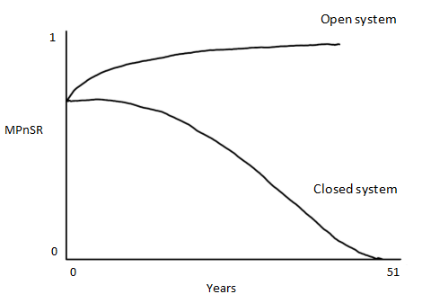
Deferrals and lump sums
Under both the pre-2016 State Pension and nSP, people can defer receipt of their State Pension beyond SPA. In pre-2016 State Pension cases, the initial entitlement was increased at a rate of 10.4% per year. If people deferred for 12 consecutive months or more, they could choose to receive a lump sum instead of the amount that they would have been paid as a pension. Therefore, the pre-2016 State Pension model had a specific component for estimating lump sums. Under the nSP, there is no longer an option to receive a lump sum and the rate at which entitlement is increased for people deferring receipt of their pension has been reduced to 5.8%.
DWP’s nSP model accounts for deferrals by calculating the caseload separately and applying a boost of 5.8% per year to the MPnSR from the year from which people are expected to take their pension. Deferral rates are estimated using FSR assumptions for deferrals, which are assumed to take place over a 10-year period and are calculated separately for males and females.
Overseas estimates
As explained previously, caseload forecasts in the nSP model are split by residency (Great Britain and overseas); and for overseas residents by whether the country of residence on retirement qualifies for annual uprating on not.
The MPnSRs for overseas inflows are calculated using a different method from that used for Great Britain (outlined previously). Instead of using L2 data for qualifying years, DWP’s model looks at historical rates of State Pensions paid to new inflows (average weekly amounts as a proportion of the full rate). These are used as the overseas MPnSR starting points, which are then trended down to zero using the same trend as for the Great Britain MPnSR.
As with the Great Britain calculation of expenditure, the final calculation involves multiplying the caseload using the following formula:
Weekly rate of nSP multiplied by weeks in a year multiplied by MPnSR
(And as with the Great Britain calculation, the expenditure is halved for inflows and exits in the year that the inflow or exit occurs).
The MPnSRs for the overseas group countries are all the same, but the final step in the calculation (expenditure) is done separately for those which are uprated and those which are not. This is because the weekly amount of the State Pension does not increase during retirement for countries with no annual uprating (that is, the increases shown in Tables 1 and 2 do not apply).
Protected payments
As explained previously, an additional complication of the nSP model is the calculation of “Protected Payments” (PPs). PPs represent an addition to the full rate of nSP if the amount that a person would have received under the old system (based on their NI record to 6 April 2016) is higher than the full rate of the nSP.
The Government Actuary’s Department (GAD) advised DWP on a “transitional calculations” model, which is used to estimate aggregate figures for PPs by single year of age and male and female split. The model applies to people aged 42 and over. It estimates “starting amounts” (SAs) and PPs on a per person basis using the L2 dataset, which includes variables associated with “contracted out” deductions (see Glossary) – the Rebate Derived Amount (RDA) and the earnings-related State Pensions, AP and GRAD.
Estimating qualifying years for the MPnSR calculation
GAD’s “transitional calculations” model used for PPs also produces estimates of “notional” qualifying years, which are those used for estimating the Great Britain MPnSRs. DWP has adapted this model when producing the national accounts figures to take account of the “minimum qualifying years” issue.
Earnings histories from the L2 dataset are used to determine the entitlement to State Pensions built up by each person in the sample in terms of qualifying years (QYs). The GAD model uses these data to calculate “notional” QYs for each person under nSP. This involves two steps:
- Notional QYs in 2016 = 35 * (SA-PP)/52.18/155.654
- Notional QYs at expected year of retirement = Min (Notional QYs in 2016,35)
DWP has added an additional step to reflect the national accounts minimum qualifying year adjustment (see Minimum qualifying years adjustment for more information). The third step – “MQY Adj” – takes the result of step 2, adds expected year of retirement (at SPA) and subtracts the year of accounts. For example, for the 2014 accounts, someone due to reach SPA in 2017 with 15.5 notional QYs in both 2016 and 2017 would have an adjustment of plus 3 years (2017 to 2014), giving them a MQY Adj figure of 18.5. However, this figure is only used to make sure that “notional QYs at expected year of retirement” are included if MQY Adj is greater than or equal to 10.
Minimum qualifying years adjustment
DWP had to build a specific adjustment into the nSP model for national accounts estimates to cope with the issue of “minimum qualifying years”, whereby people need at least 10 qualifying years to receive any State Pension. As discussed previously, for the national accounts work, the long-term projections models designed for fiscal sustainability analysis had to be adjusted to remove any accruals beyond the date of the accounts. However, this meant that if people had accumulated fewer than 10 qualifying years at the date of the accounts, they were automatically eliminated from the estimates. Among other things, this eliminated a whole generation of young people who had not yet worked for 10 years, most of whom would in fact go on to meet the “minimum qualifying years” requirement.
Eurostat provided guidance on such cases, suggesting that individuals with fewer than 10 years’ entitlements accrued should first be modelled according to the probability of completing 10 years in future; then those expected to complete 10 years should be given a value representing the proportion of the total pension accrued at the date of the accounts. DWP therefore made an adjustment to the nSP model (known as “MQY Adj”), comparing the number of qualifying years of each person in the L2 dataset at the date of the accounts with the number of qualifying years at their expected “year of retirement” (SPA). If adding a qualifying year for each year up to and including their year of retirement gives them greater than or equal to 10 qualifying years, then the person is given a value representing the proportion of the total pension entitlement accrued at the date of the accounts (that is, the fact that they have not yet met the “minimum qualifying years” requirement is ignored). If they will have less than 10 qualifying years by SPA, they are given a value of 0 entitlement.
Limitations of the nSP model
This section lists some known areas of weakness in the nSP model. These are either due to lack of data or to decisions having been taken to simplify approaches due to resource constraints:
overseas caseload forecasts are a snapshot of the situation as at SPA; there is no information about people moving overseas (or back to UK) after SPA
overseas MPnSRs are not based on the “transitional calculations” methodology developed by GAD; the reason for this is that there is insufficient information on qualifying years for this group in the L2 dataset
with the introduction of nSP, new models are required to forecast the decay of lump sum and AP expenditure respectively; these models switch off both inflows and accruals in 2016 and due to resource constraints, DWP has used the outputs of the FSR16 models (as produced for FSR16) for the 2014 and 2015 accounts figures
Notes for: Column H: The new State Pension model
A GB to UK uplift factor is applied produce estimates for the UK.
The explanation in this section is based on the treatment of Great Britain inflows. Overseas inflows are estimated differently.
51 = 67 – 16 because the SPA of the youngest working person was 67 years under the legislation in place in 2015 and their age was 16 years.
35 = total number of years required for full state pension under the new system; 52.18 = number of weeks in the year; £155.65 = weekly rate of nSP in 2016.
Category B pensions are those based on a spouse or civil partner’s contribution record.
12. Column H: Changes affecting both models
Updates of source datasets
The source datasets used by DWP in its models are:
for the pre-2016 State Pension, BSP and GRAD models (“pensioners” part of the model), the Quarterly Statistical Enquiry (QSE), a biannual 5% sample of administrative data
for the pre-2016 State Pension, BSP and GRAD models (“inflows” part of the model): the L2 dataset (a 1% sample of HM Revenue and Customs’ National Insurance Recording System)
for the pre-2016 State Pension, AP and lump sums models: the L2 dataset
for the nSP model: the L2 dataset is used both to calculate MPnSRs and PPs
ONS’s population projections and information on mortality, marital status and widowhood are also used in both models (although marital status and widowhood are no longer needed for the nSP model).
In principle, the model uses the relevant year’s dataset and should move on by one year of data for each year of accounts. However, in some cases this was not done due to issues with the source data. The updates of the datasets feed into the way the model produces estimates of entitlements accruing each year. Therefore, it is possible that the estimates of accruals have been affected.
Updates of economic assumptions
The important economic assumptions that have to be updated every year are the uprating (benefit indexation) and wages or earnings growth assumptions. For uprating, DWP uses the assumptions published in the OBR Economic and Fiscal Outlook (EFO) Table 4.1: Determinants of the fiscal forecast for the short term and in the OBR’s fiscal sustainability report for the long term. Wage growth assumptions come from EFO supplementary economy Table 1.6 and the CPI assumptions from Table 1.7. In years when actual uprating figures were available at the time of modelling, these were used instead of the EFO assumptions.
Order of changes
For Table 29, ONS requires not only estimates of liabilities (opening and closing balances) but also estimates for the specific in-year changes (see Section 13). The order in which the estimates are calculated affects the results for in-year changes. It was decided (on advice from GAD) when producing the estimates for the 2010 table that the following order worked best:
- change due to demographics
- change due to update of economic assumptions (including changes in uprating)
- change due to re-evaluation of liabilities as discount factor moves on a year
- change due to payment during year
- change due to update to data or additional year of accruals
- change due to model updates
- change in scheme rules: reforms other than SPA changes
- change in scheme rules: changes in SPA
In 2011 and 2012, however, the order was changed. In particular, economic assumptions changes came towards the end, after update of data or additional year of accruals. This may have affected the estimate of how much of the change in liabilities between the start and end of the year was due to each component in the hierarchy.
Model updates
In 2013, some problems were identified with the code used in the pre-2016 State Pension model. These were rectified, producing a large change in State Pension liabilities or entitlements due to “model updates”. The corrections to the code relate to:
amending the method of calculation for qualifying years, linked to the updating of the data from L2 2010 to L2 2015 in the 2013 accounts
correcting an error in the calculation relating to the accrual of Category B pensions
correcting an error in a section of the SPA code
13. Column H: Using the model outputs to produce Column H
Column H presents estimates for accrued-to-date entitlements or liabilities of social security pension schemes (State Pensions in the UK) and the associated flows of money in and out of the scheme.
The opening and closing balances are shown in Rows 1 and 10 respectively and must be calculated on an actuarial basis using a nominal discount decided by Eurostat, which is currently 5% (it has remained at this level since the first table was published by ONS, for 2010). These figures are calculated by DWP’s pre-2016 State Pension and new State Pension models.
The in-year changes between the opening and closing balances are shown in the rows in between (Rows 2 to 9). These include:
- the “transactions” rows, which show actual and supplementary contributions and benefits (Rows 2 and 4) and the impact of policy changes and reforms on past service cost (Row 7)
- the “other economic flows” rows, which show the value of changes in the actuarial assumptions used to calculate direct benefit (DB) pension entitlements (Rows 8 and 9)
- the “residual” or balancing item after all transactions and other flows have been accounted for (Row 3)
The “transactions” rows
Rows 2.1 and 2.3 contain estimates of actual NI contributions paid by employers and employees in respect of State Pensions; the split is estimated using the percentage of National Insurance Fund benefit payments going to State Pensions.
Row 2.4 is the “unwinding of the discount rate”, or revaluation of liabilities between the start and end of each year, which is calculated by multiplying Row 1 by the nominal discount rate set by Eurostat.
Row 4 shows the payment of pension benefits during the year. These figures are calculated by DWP’s pre-2016 State Pension and nSP models.
Row 6 shows transfers of pension entitlements between schemes, which are negligible in the case of State Pensions and are assumed to be zero.
Row 7 contains an estimate of changes in “past service cost” (that is, benefits accrued in previous years) due to legislation enacted during the year in question and official announcements made during the year. These are also known as changes due to reforms, or negotiated changes. These figures are calculated by DWP’s pre-2016 State Pension and nSP models, taking into account any legislation enacted in the year in question that affects pension entitlements, even if the changes take place in a future year.
The “other economic flows” rows
Rows 8 and 9 come from the DWP model outputs for the pre-2016 State Pension and nSP.
Row 8 shows any changes in entitlements due to changes in financial assumptions including discount rates, wage growth, indexation of benefits and inflation. It is well known that changes in the discount rate have major impacts on liabilities and any such changes would be recorded in Row 8, but as the discount rate has remained at 5% since the 2010 table was published, there are no changes due to the discount rate recorded in Row 8 in the 2010 to 2015 period. However, the other financial assumption changes can also have significant impacts. For instance, DWP’s models estimate that in 2015 changes in uprating assumptions (in particular, the long-term assumption for indexation of benefit payments, which fell from 4.89% to 4.64%) resulted in a £265 billion decrease in the value of accrued-to-date liabilities.
Row 9 shows any changes due to other assumptions, mainly changes in demographic assumptions such as life expectancy. In 2014, the DWP State Pension models moved from using ONS’s 2012-based population projections to its 2014-based projections, which had higher age-specific mortality rates. The reduction in the value of accrued-to-date liabilities due to increased mortality was estimated at £149 billion.
The residual row
This row is calculated simply as the closing balance minus the opening balance, minus all transactions and other economic flows that can be accounted for during the year. It captures:
any “surplus” (negative sign) or “deficit” (positive sign) building up during the year where National Insurance (NI) contributions are higher or lower than the amount required to meet the accruing entitlements to future State Pensions (increase in liabilities)
the amounts accruing for people who may not earn enough to make NI contributions but are credited with qualifying years, which allow them to build up State Pension entitlements (positive sign)
experience effects, where outcome of modelling differs from the assumptions (negative or positive sign)
model changes, updates or corrections (negative or positive sign)