1. Introduction
Official statistics such as those published by the Office for National Statistics (ONS) and the wider Government Statistical Service (GSS) inform on many important themes in society such as the social and demographic composition of the population, the economy, the environment, health, education and housing among others. Official statistics are fundamental to the judgements and decisions made by government, industry and the wider public and are an essential public asset for planning resources and monitoring the economy and welfare of citizens.
These statistics have traditionally been based on surveys or censuses. A census – a count of all people and households – is undertaken by ONS every 10 years and provides the most complete source of information about the population that we have. It is unique because it covers everyone at the same time, which provides an accurate reference base for many statistical series such as population estimates and projections and sample surveys. Complete and accurate address information is critical to the operational design, planning and delivery of ONS social surveys and Census, as it forms the underpinning frame for collection. In addition, many of the statistical outputs rely heavily on geographical references linked to addresses.
ONS is seeking to increase the role of administrative and other data sources in the production of official statistics as part of its “Better Statistics, Better Decisions” strategy. Accurate geographical referencing is vital to making such data compatible and comparable with existing datasets and outputs. Similarly, departments across government and the public sector find themselves in need of standardising the geographical information across their datasets to enable them to deliver better insight, service or policy outcomes. Ideally the geographical reference would be assigned once at the time of data collection. As ONS is starting to take advantage of electronic questionnaires, especially for the 2021 Census, it requires a service providing real-time address matching. The address index (AI) project aims to satisfy this need through delivering a highly accurate, reliable and scalable address matching service.
This paper describes the methodology which underpins the address matching process behind the AI and shows its performance. The background focuses on a general overview of the task at hand. Sections 3 to 6 describe the data processing pipeline, algorithms used and performance measures. Finally, we discuss the benefits and shortcomings of the current service and possible future steps.
Back to table of contents2. Background
Address matching is an example of a broad class of data science problems known as data linkage. The common aspect of all these problems is that they require an association between data (commonly two sources) to be devised based on some common property of the data. For address matching, the common property is the address itself but, given that there is no universally accepted standard for the “correct” form of the address, and sources commonly store address data in many different forms, matching addresses becomes a significantly complicated task.
The objective of the address index (AI) project is to tackle the issue of there not being a universally accepted standard for what constitutes the correct address for any building or place in the UK, and to develop a methodology which provides high quality outcomes regardless of the input.
Reference data for address matching
The Ordnance Survey product AddressBase (AB) aims to provide comprehensive up to date address information combining two data sources: the National Address Gazetteer and Royal Mail’s Postcode Address File (PAF). Each record in AddressBase is equipped with a persistent unique identifier called unique property reference number (UPRN) which provides a reference key across different Ordnance Survey datasets. This is important as this allows for alternative property names (for example, in Welsh language) whilst avoiding duplicate records within one dataset. Address information is well structured and divided into individual address components (for example, building number, town name, postcode) while keeping reference to the original data source (National Address Gazetteer or Postcode Address File). The records aim to be as complete as possible which is not necessarily the way people usually write their addresses. Quite often people use acronyms and omit parts of the address such as locality or postcode. On the other hand, business names are not commonly present in AB.
The AI service will provide a single consistent form (and UPRN) for any free-form address that a user enters and will allow users to identify an address based on incomplete information that they have available. Table 1 provides a summary of the linking problem:
Table 1: Overview of the address linkage problem
| Input address string | Reference data to match against (AddressBase) |
|---|---|
| Unstructured text | Structured, tokenised |
| Messy, containing typos etc. | Complete & correct (more or less) |
| Incomplete | Snapshot of addresses at a given time |
| Range from historic to very recent addresses, including businesses | Organisation / business names are not always part of the address |
| Source: Office for National Statistics | |
Download this table Table 1: Overview of the address linkage problem
.xls (37.9 kB)Address matching pipeline
The address matching process can be split in three high level steps, which are described more fully in their own sections.
Address parsing
Splits the input address string into appropriate address components. For this purpose, we train a classification algorithm (conditional random fields), and we also implement strategies to handle cases that are not perfectly parsed.
Candidate address retrieval
Quick and scalable system to identify a subset of AB addresses that are relevant to the input address. This has been implemented using Elasticsearch with fine-tuned query and postprocessing of the relatively small pool of returned addresses.
Ranking and scoring
The service returns an ordered list of candidate addresses (and UPRNs) including a measure of confidence in the presented results.
The performance of the whole matching system depends on each step. Each step has been optimized on its own as well as in combination with others as the focus is on the overall performance of the whole service. We have adapted standard evaluation measures to the specific address matching task. This allow us to monitor the progress throughout the system development as well as benchmark it against other address matching services.
Back to table of contents3. Address parsing
Given that the reference AddressBase (AB) data provides the addresses divided up into different address components while the input is one text string, there are potentially two ways to prepare the data to enable comparison. The input string can be broken up into corresponding address components that can be matched individually against the AddressBase data. Alternatively, the AddressBase records can be concatenated to produce an address string that can be compared against the whole input string. Both approaches have their advantages and therefore both are used in the matching process.
Tokenisation
The process of parsing the input string and selecting the words which correspond to building name or number, locality, town name, postcode, and so on is called tokenisation. This allows for more accurate comparison because comparing tokens precludes the possibility of the same word representing one element of the address being compared against an unrelated element of the address. For example, without tokenisation a road name like “Essex Road” could be successfully matched against an address like ”12 Park Road, Harlow, Essex” because “Essex” and “Road” occur in both address strings. However, when the addresses are broken up into tokens, the road name from the input string is only compared with the road name field in the reference data and thus the above would not be matched.
Tokenisation is not a simple procedure since it requires the address to be accurately split into words in the first place and then the words to be labelled using the same schema as in the AddressBase data sources. Splitting up an input address can be complicated because, for example, some people may use a hyphen or comma to divide up the words while others may use only a space.
In practice, while tokenisation is not infallible, it can be time intensive when it requires someone to decide what constitutes a sensible rule and what does not. There is also the added complication that AddressBase has been generated by humans deciding how to label the different words of the address.
Concatenation
In contrast to tokenisation, concatenating (joining) pre-existing tokens to reproduce an address is trivial, and it also removes the need for complicated tokenisation of an arbitrary address string. Unfortunately, concatenation destroys some of the information in the data about the address, namely the labels identifying the part of the address that the word represents. Neglecting this information makes the matching more difficult as two addresses might be similar semantically but have different syntax. It makes it impossible to rely on the natural structure of the address to help match the desired address with the input string. However, for input strings with unusual structures, tokenisation might be impossible and comparison of the full address string still provides a valid result.
Parsing algorithm
The requirement to maximise the match rate meant that tokenisation would have to be used. Given that there is limited control over how the address is entered (one of the requirements is that the address index (AI) should be able to match an address input without any constraints on how the address should be formatted) the parser must be flexible enough to deal with free text. There are two broad approaches to doing this:
- rule-based parsing
- structured learning
Rule-based parsing uses a set of deterministic rules that are derived by a human based on their research and experience. Usually, the rules are implemented in a programming language (SAS has been used in the past for address parsers in Office for National Statistics (ONS)) which goes through each address systematically and applies the rules that form the program. Given that parsing is usually done without any human intervention, the rules aim to be exhaustive but can lead to odd results for addresses which do not neatly conform with the rules. This leads to many rules and interdependencies that become unmanageable and inflexible to input variations. The alternative is to use a structured learning approach.
Structured learning is a catch-all term which describes how a computer can automatically generate a method of parsing based on meeting an objective for all the elements of a data set. In principle, an algorithm could be developed which would generate a model that could be deployed to accurately parse any given address string. In practice, the number of possible address strings is effectively infinite (it is possible to generate several variants of an address by transposing elements of the address, changing spellings, excluding certain words, and so on) so the model needs to be developed to only consider likely input strings and a certain failure rate needs to be accepted in order to make such a model tractable. The major advantage of structured learning techniques is that they require only limited human intervention and can be rerun if the underlying data changes without having to undertake a complicated update project.
As part of the discovery process, a number of structural learning algorithms were investigated to compare their strengths and weaknesses. The alternatives considered were:
- Conditional random fields (CRF)
- Hidden Markov model
- Maximum entropy Markov model (PDF, 116KB)
- Transformation-based learning (brill tagger)
- Averaged perceptron
- Structured support vector machine
The outcome of the investigation was to use conditional random fields (CRF), over the other methods, because of its high predictive power, rapid execution speed at runtime and readily available implementation with minimal additional dependencies. For a given token, CRF uses information about the label applied to the previous token and the features associated with the current token to determine what the most likely label is for the token under consideration. Figure 2 shows an intuitive representation of how the CRF works.
Figure 1: Visualisation of the CRF classifier on address string

Source: Office for National Statistics
Download this image Figure 1: Visualisation of the CRF classifier on address string
.png (88.7 kB)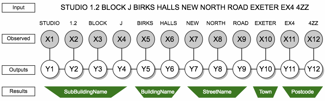
In the above diagram, each of the words is represented as an input element X1, X2, X3, ..., X12 and the labels attached to each word are represented by Y1, Y2, Y3, ..., Y12. Therefore, the output of the CRF model to the inputs gives a string of labels which are interpreted as building name, street name, town, etc. Note that the input elements consist not only of the words themselves but also of a list of “features” that give information about the word, such as: whether it contains digits, if it is a synonym for “flat”, whether the previous word contains digits, whether the following word is a synonym for ”street” and so on. The features and synonyms lists included in the model were proposed based on subject matter expertise and evaluated based on their discriminatory and predictive strength in the model. Further details on the selected features can be found in Appendix I.
CRF models have the great advantage of not requiring any detailed knowledge about the probability of any of the features occurring as, for example, hidden Markov models do. As a result, CRF models are ideally suited to address parsing. The CRF model has been trained on a random subset of addresses from AddressBase. The names of AB fields were used as training labels and the addresses were augmented to reflect imperfections of the real input address strings. To improve the classification, larger training weights were assigned to underperforming minor types of addresses, for example, Welsh language versions. The trained CRF model has achieved more than 98% accuracy, that is, for 98% of address strings the whole sequence was correctly split into the address elements. The address element with most misclassification (around 20%) was department name, mostly because of its low frequency and consistency in training dataset.
Back to table of contents4. Candidate address retrieval
Having handled the issue of how to turn an input address string into a set of tokens that can be matched against the address fields in AddressBase (AB), a method to compare the input tokens against all the AB addresses was required. Our approach makes use of the Elasticsearch information retrieval engine to deliver quick searching through the AB database. Elasticsearch is a fast, highly scalable open-source full-text search and analytics engine. It allows for complex search features and requirements, which makes it the ideal underlying technology for the address index (AI).
The following steps are taken to retrieve the best matching candidate addresses.
Step A: Each parsed token of the input address is compared against relevant AB address fields
Each address component (such as the building number) identified by conditional random field (CRF) is matched to all the AB fields that could contain that element. This allows us to compare input against different versions of the address, for example, a Welsh one. It also mitigates against some common parsing errors, for example as locality and town are often ambiguous in the input, it allows for matching across multiple fields.
Step B: Matches allowing for synonyms and fuzziness
A custom list of synonyms has been derived based on domain expertise, including acronyms and commonly interchangeable terms, for example “apt ~ apartment ~ flat”. Fuzzy matching refers to allowing a non-exact match between the strings, for example “Birmingham ~ Birmingam” is one letter different (using Levenshtein edit distance). A perfect match receives a higher score than a fuzzy one, but allowing a limited fuzzy search deals with imperfections of the input such as typos and misspelling.
Step C: Combining and “boosting” scores of the individual matched fields
This step combines the scores calculated for each pair “parsed token / AB field” from Step B. If there is a match of one parsed token to more than one AB field (for example, in AB a building number can be stored in a number of fields resulting from the underlying data used to build AB), we take a maximum of the individual scores, so called dismax function in Elasticsearch. It is a natural operation for this situation as the score interpretation here would be “does the building number match to any of the AB building number fields?” and it does not matter whether the match has been found in the English or Welsh version of the address in the National Address Gazetteer fields or Postcode Address File fields. Each individual match field also has a “boost” associated with it, which is used to multiply the score in order to give more importance to some fields over others. The initial design for the logic to combine the token comparison and associated weightings was generated through discussion with subject matter experts and experimentation.
Step D: Fall-back query on full address and bigrams
Alongside the structured comparison described above, an unstructured search is performed, such that the whole input string is compared with a concatenated version of the AB address. It receives a score calculated using TF-IDF based metric that quantifies how well the whole strings match (see Appendix II). The score is calculated for matching individual words as well as pairs of consecutive words, bigrams. The usage of bigrams mitigates the risks of matching wrong parts of the address together. Again, a boost is used to optimize weight or importance of match in these fields. However, as we would expect only a small proportion of addresses to fail to be parsed accurately, the boost for this fall-back query is small.
Step E: Minimum match threshold
Up to 40% of the parsed tokens from the input address are tolerated to be unmatched against the AB reference address in order for the candidate address to still be returned by Elasticsearch. It is implemented using a “should” clause with the required minimum match threshold and it is applied to the structured component-wise query as well as the fall-back one. This is a first filter removing less suitable candidates, later a stricter one is applied outside of Elasticsearch.
Step F: Final Elasticsearch score
All the AB addresses that are matched on at least the minimum number of tokens are considered possible candidate addresses (Step E). The final Elasticsearch score is calculated by summing up the fall-back score from Step D with the scores for all individual tokens (Step C), because a match in each address component contributes to how sure we are that the whole address is a correct match. Elasticsearch returns the candidate addresses ordered by this score. The raw values of this score are not comparable for different inputs, but they feed into the calculation of our custom confidence score.
The Elasticsearch query configuration and associated parameters have been optimised step by step using input datasets provided by potential customers. A detailed diagram illustrating which parsed tokens are compared to which AB address fields and how they are combined together can be found in Appendix III.
Back to table of contents5. Scoring and ranking
The last step in the process is to evaluate and convey quality of the match between the input and the retrieved candidate address (its unique property reference number (UPRN)) in such a way that would be easily understood and useful for users. A percentage has been found to be most popular option because it combines an intuitive measure (people understand how good 65% is) with something that allows automatic filtering to cut off the end of a results set.
Bespoke score
Depending on the type of address different amount of information in the input may be required to confidently resolve the best match. For example, postcode and building number combination can uniquely identify around 85% of residential addresses, but a perfect match at a building level can be ambiguous at the unit level (where a building might contain several flats or units for example). A deterministic bespoke scoring system has been devised that reflects a subjective expectation based on experience and subject expertise. A pair “input / candidate address” gets assigned to predefined category based on which tokens are available in each of them and how well they match. Each category scores between 0% and 100%. There are a large number of possible combinations so the tokens are grouped and evaluated at three levels: locality, building and unit. An overview of categories and associated scores can be found in Appendix IV.
This bespoke score has the advantage over Elasticsearch score that it conveys the intuitive measure of confidence and is tailored to the format of UK addresses. On the other hand, the disadvantage is that it does not deal with imperfect parsing and does not incorporate information about other candidate addresses (such that if there are no other candidates then even a mediocre one is likely to be good enough, while if there are several mediocre ones then we cannot be confident about any of them).
Confidence score
Reporting multiple scores (elastic and bespoke scores for each of building, locality and unit) would only create user confusion. An investigation has been undertaken to explore possible models to calculate a single confidence score using currently available information such as the Elasticsearch score, the bespoke score and its categories, token properties and the difference or ratio of scores between candidates. The task at hand is a binary classification, where we are interested in the probabilities accompanying the predicted class label (true match vs incorrect candidate address). The classifiers considered were:
Feature selection was done using:
The best indicator of whether a candidate address is indeed the correct UPRN is the Elasticsearch score ratio. It is calculated by taking the Elasticsearch score of the candidate in question and dividing it by the sum of the two best scores for the input string. It results in a value between 0 and 1 that can be translated into a percentage with highest values achieved by candidates that receive significantly larger Elasticsearch score than the next best candidate. Nevertheless, there are cases where the independent bespoke score brings additional information – the intuitive “confidence” number. As we prefer to keep candidates that have received a good score from either of the two methods we propose an ad-hoc simple confidence score calculated as a maximum of the two values (after appropriate scaling, see Appendix IV). This simple confidence score was benchmarked against the above mentioned classifiers and it has achieved comparable results as measured by standard metrics such as accuracy, F1 score and AUC (area under receiver operating characteristic (ROC) curve). It has the additional advantage of being interpretable and simple to implement and therefore it was adopted as the main confidence score.
Ranking and thresholding
For each address string, a short list of candidate addresses (UPRNs) has been identified and the above defined confidence score calculated for each of them. The results are sorted in decreasing order by the confidence score and in case of equal confidence scores, the UPRN is used as secondary key. Based on the users’ preferences the least relevant results are removed from the list, that is, the candidates with confidence score below a chosen threshold are discarded. The threshold value varies depending on the user case. For example, if an individual match is requested and reviewed by human, a good threshold would be 5% because it allows more candidates to be displayed if there is any ambiguity. For a purpose of automated matching, only very good matches should be returned and therefore the recommended threshold is 60% to 80%.
Back to table of contents6. Performance evaluation
Evaluating the performance of address index (AI) is not as straightforward as it may seem. For an input address, the service returns one or more candidate unique property reference numbers (UPRNs) (with attached confidence score). We are looking for a fine balance between offering enough possible candidates but on the other hand not including too many loosely similar addresses.
Baseline datasets have been obtained from various sources, taking into consideration potential customers and their needs. Some of them consisted of a list of address strings while others included the reference UPRN. Through the development, we monitored the performance using six datasets containing in total around 200 thousand labelled and 30 thousand unlabelled records.
Test data with UPRN (labelled)
For each address, the comparison between true UPRN and candidates' UPRNs results in one of the four cases:
Top match: The best scoring UPRN matches the ground truth. In order to be considered top match its score has to be strictly greater than any other candidate's.
In the set: The true UPRN appears within the five highest scoring candidates but not as the unique top match.
Not found: This is the case when AI does not return any candidates.
Wrong match: One or more candidate UPRNs are returned but the true one does not appear in the top five.
Our goal is to maximize the number of top matches while keeping the number of wrong matches (false positive rate) acceptably low.
The quality of input data is highly variable across the datasets and so is the matching performance. It is therefore impossible to pre-set any acceptance criteria for the matching performance or to quantify all four categories into one cost function. Instead we always report the proportion in all four categories and monitor changes in performance in the form of movement between them.
Test data without UPRN
Without the true UPRN available there is nothing to compare the candidate against and we can only measure the proportion of addresses in the following two categories:
New UPRN: Possible match is returned.
Both missing: No candidates are offered by AI.
Additional clerical resolution would be required to valuating the false positive rate in this case.
Current performance
Table 2 shows how many of the records fall in each of the above defined categories.
Table 2: Matching performance of all baseline datasets combined
| Performance category | Number of cases | Percentage | |||
|---|---|---|---|---|---|
| input with UPRN | 1 top match | 193681 | 97.50% | ||
| 2 in set | 2248 | 1.13% | |||
| 3 not found | 51 | 0.03% | |||
| 4 wrong match | 2659 | 1.34% | |||
| input without UPRN | 5 new UPRN | 28391 | 99.86% | ||
| 6 both missing | 41 | 0.14% | |||
| Source: Office for National Statistics | |||||
Download this table Table 2: Matching performance of all baseline datasets combined
.xls (39.4 kB)Note that more than 97% input addresses are matched to the correct UPRN. In less than 2% cases, the AI fails to provide good candidates and in the remaining cases the user needs to choose from a list of candidates.
Measuring change in performance
We attempt to objectively quantify the change in matching performance in order to compare methods and measure the impact of proposed improvements. Ideally, we want to increase the number of top matches and decrease wrong matches simultaneously on ALL types of input (represented by our six datasets). That is not always possible and a big gain on one dataset might result in a loss on another one. For each step during the development, we had carefully weighed the gains versus losses and discussed these with the experts in the Office for National Statistics (ONS) Address Register team.
The matching performance of the AI service has been benchmarked against similar commercially available solutions. It has outperformed the alternative services in the total number of matched addresses as well as in the quality, that is, based on clerical resolution the addresses (and UPRNs) provided by AI were correct in more cases than the alternative services. For example, ONS Life events team uses a commercial postcode finding tool in their data processing pipeline. We have compared its matching performance with AI service using more than 11,000 addresses from their actual dataset. Based on their acceptance criteria the external tool provides UPRN automatically for 80 to 85% percent of the records. The remaining ones need to be resolved manually and that is costly. In comparison, the AI service provided 96% of UPRNs automatically and therefore it would lead to significant reduction of cost. Note that in most cases (90%) both services came up with the same UPRN, but out of the remaining cases: 80% of time AI provided the correct UPRN, in 10% the external matching service was correct and the remaining 10% was inconclusive (usually due to low quality input). This shows that the AI index leads to cost reduction and quality improvement at the same time.
Back to table of contents7. Conclusion
The address index (AI) project has delivered an address matching service that meets the need for assigning geographical references to many datasets. The quality of the provided matches is very high in absolute terms, as well as compared to existing methods and commercially available tools. The actual implementation of the methodology outlined in this paper uses innovative data science methods and tools, that make the service reliable and scalable, but technical details (such as infrastructure or security) are beyond the scope of this paper. As the service is gradually being used by more customers new requirements have arose. For example, we are currently looking into offering search-as-you-type functionality and a “time machine” to allow users to search historic versions of addresses from a particular time period. The methodology and code are being open-sourced to enable interested parties to have confidence in the service, as well as permit re-use across government and potentially internationally.
Back to table of contents9. Appendix
I. Features used in conditional random fields model
The features used in the CRF model are:
Digits - all, some or no
Word - word (for example, New) unless the word contains digits, in which case it is False
Length - length of word or digits
Ends in punctuation - True / False
Directional - True / False - word is one of N, E, S, W, NE, NW, SE, SW, North, South, East, West, Northeast, Northwest, Southeast, Southwest
Outcode - True / False – for example, AB10
Post town - True / False - for example, Aberdeen
Flat - True / False - word is one of Flat, Flt, Apartment, Appts, Appt, Apt, Room, Annex, Annexe, Unit, Block, Blk
Company - True / False - word is one of CIC, CIO, LLP, LP, LTD, Limited, CYF, PLC, CCC, Unltd, Ultd
Road - True / False - word is one of Road, Raod, Rd, Drive, Dr, Street, Strt, Avenue, Aveneu, Square, Lane, Lne, Ln, Court, Crt, Ct, Park, Pk, Grdn, Garden, Crescent, Close, Cl, Walk, Way, Terrace, Bvld, Heol, Ffordd, Place, Gardens, Grove, View, Hill, Green
Residential - True / False - word is one of House, Hse, Farm, Lodge, Cottage, Cottages, Villa, Villas, Maisonette, Mews
Business - True / False - word is one of Office, Hospital, Care, Club, Bank, Bar, UK, Society, Prison, HMP, RC, UWE, UEA, LSE, KCL, UCL, Uni, Univ, University, Univeristy
Locational - True / False - Basement, Ground, Upper, Above, Top, Lower, Floor, Higher, Attic, Left, Right, Front, Back, Rear, Whole, Part, Side
Ordinal - First, Second, Third, Fourth, Fifth, Sixth, Seventh, Eighth, 1st, 2nd, 3rd, 4th, 5th, 6th, 7th, 8th
Hyphenations - Number of hyphenations
Vowels - True / False - Whether the word contains vowels
Raw string start / end - word is at the start or end of the string - True / False
Table 3 gives examples of the most discriminative features. It means that if a word in the input has the property listed in the left column then it is more likely to be labelled as the corresponding address component in the right column. While the features were manually selected, the strengths of these associations have been learned by the CRF algorithm automatically during model training.
Table 3: Examples of discriminatory features used in conditional random field (CRF) model
| Feature | Label (Address Component) |
|---|---|
| Word: ‘NEW’ or ‘GREAT’ or ‘ST’ | Town name |
| Previous word: ‘LITTLE’ | SubBuilding or Building name |
| Raw string end | Postcode or Locality or Town name |
| Some digits | Postcode |
| Next word: ‘INDUSTRIAL’ | Locality |
| Source: Office for National Statistics | |
Download this table Table 3: Examples of discriminatory features used in conditional random field (CRF) model
.xls (38.4 kB)II. TF-IDF based similarity for addresses
Similarity between two address (or address components) strings is calculated using the underlying Lucene similarity function which is based on cosine distances between TFIDF weighted document vectors. The TF-IDF based similarity function is beneficial for cases such as in “Obscure Street” because the word obscure gets higher weight as it is specific in comparison to street – a more generic term. On the other hand, why should “Some Street, London” have lower score than for “Some Street, Pontrhydfendigaid” assuming no town is in the input? To make the scores more comparable between each other, we wrap the individual match clauses in the structured part of the query in “constant score”.
III. Elasticsearch query diagram
The download attached (xls, 16.0KB) illustrates which parsed tokens are compared to which AB address fields. The names of the fields in the diagram are taken from AB record structure, where prefix “‘nag” is used for address information contained in National Address Gazetteer (Local Property Identifier as well as Street Descriptor) while “‘paf” refers to Postcode Address File.
IV. Bespoke scoring matrix
The rules of the bespoke scoring system can be found in the attached Excel spreadsheet: Bespoke scoring matrix (xlsx,112 KB).
V. Confidence score scaling and thresholding
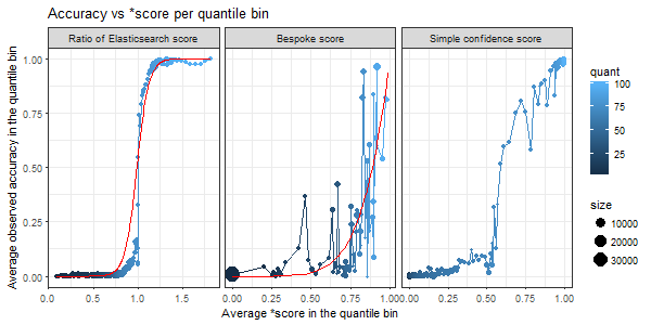
To make the Elasticsearch score and the bespoke score comparable we need to scale them, ideally to match the observed accuracy. In the picture below, each blue dot represents a group of input addresses with the average score per the group on x- axis and average observed accuracy on y- axis. Each group correspond to a quantile bin on the score in question. Ideally, these blue dots should lie on a 45-degree line. The proposed monotonic transformations that should achieve that is shown as a red line, for the Elasticsearch score ratio it is a sigmoid while for bespoke score a power function.
Figure 2: Various scores compared to observed accuracy
Source: Office for National Statistics
Download this image Figure 2: Various scores compared to observed accuracy
.png (27.8 kB) .xlsx (42.1 kB)
The recommended 5% threshold on simple confidence score is based on the following observation, that has been found desirable across the baseline datasets:
- for addresses in 1_top_match category we drop 54% candidates (while never actually dropping the correct match)
- for addresses in 2_in_set category we drop 21% candidates, while losing less than 5% correct matches
- over all categories we would drop 53% and lose .06% of correct matches
VI. Implementation notes
The code is publicly available in github: address index data and address index api.
Back to table of contents