1. Introduction
Official statistics are published by governmental and other public bodies and inform the public on many important themes in society such as the social and demographic composition of the population, the economy, the environment, health, education and housing, among other things. Official statistics are an essential public asset. They are fundamental to the judgements and decisions made by the public, by government and by an enormous range of other organisations.
These statistics have traditionally been based on national surveys or censuses. A census – a count of all people and households – is undertaken every 10 years and provides the most complete source of information about the population that we have. It is unique because it covers everyone at the same time, which provides an invaluable reference base for many statistical series such as population estimates and projections and sample surveys. More recently, the data sources include operational data collected by government in the administration of its services, such as welfare, tax records and General Practitioner patient’s register, among other things.
With the aim of reducing data collection costs, the government is seeking to increase the role of administrative and other new forms of data, including that found in the private sector, generated from sensors or available on the internet. Earth Observation (EO) data include satellite and aerial imagery and are emerging sources of data relevant to several areas of official statistics, for example, land use, agriculture and transport. The EO use cases include urban geospatial planning, environment and forest monitoring as well as monitoring of fish stock, ice and marine environment. In inaccessible regions, the EO science makes significant contributions in the food security and disaster risk reduction sectors. Using the EO data would enrich our understanding and options in measuring related phenomena and could potentially lead to more timely and accurate statistical products, while reducing the cost (frequency and response burden) of surveys.
The Office for National Statistics (ONS) Big Data Team explored the potential of satellite and aerial imagery in the production of official statistics through a small pilot project using publicly available Google aerial images of UK addresses. The aim was to assess the ability of machine learning techniques to detect residential features of interest, such as caravans and clusters of similar housing. As well as providing experience in acquiring, handling and analysing satellite imagery data, the pilot assessed the feasibility of using these data to enhance intelligence on addresses currently available to ONS, in particular within the AddressBase.
This article compares several classification methods to detect caravan parks, for example, Gaussian Naive Bayes, Logistic Regression, Support Vector Machine and Random Forest. The main focus is on the results from the most accurate method: artificial neural networks. Section 2 provides background information on EO data and the AddressBase, section 3 outlines the data, analysis and results of the pilot and section 4 provides a list of further literary resources.
This pilot aimed to demonstrate whether intelligence on caravan park addresses could be extracted from aerial imagery using freely available Google aerial images.
Back to table of contents2. Background
A primary objective for the Office for National Statistics (ONS) Big Data Team is to assess how evolving data sources and data analytics could be used to improve the production of official statistics. One such data source, Earth Observation (EO) data, includes satellite and aerial image data and is increasingly available for the UK. This rich source of information has broad potential to provide geospatial intelligence that might improve the information ONS holds about addresses. This information is essential for carrying out surveys and the census.
Earth Observation data
Earth Observation (EO) data comprise information needed to measure, monitor and predict the physical, chemical and biological aspects of the Earth system. They include measurements taken by various technologies including remote sensing platforms such as satellites, manned and unmanned aircraft. Some of the specific applications of these data include forecasting weather, predicting climate change and environmental impact, and monitoring and responding to natural disasters, including fires and floods.
The availability of satellite imagery is undergoing fast development with improvement of the quality and resolution as well as the frequency. The amount of available timely data is growing and costs for these data are falling at the same time. Copernicus, the European Programme for establishing European capacity for EO, has a system of Sentinel satellites producing a variety of earth images that are available at no cost. Coming in a variety of specifications1, the extended spectrum images can be used for determining detailed analysis such as soil or crop type and land use. Other free sources of EO data include ArcGIS and Google maps, which can be downloaded using an application programming interface (API)2. These data were assessed within the pilot as they provide standard aerial photography, already pre-processed and more easily accessible.
AddressBase
Complete and accurate address information is critical to the operational design, planning and delivery of ONS social surveys and the census. Many output statistics, including census outputs, rely heavily on geographical references linked to addresses. To meet the needs of the 2011 Census, ONS built a national household address register for England and Wales (PDF, 170.8KB), which combined address information from several existing sources, including Royal Mail, Ordinance Survey and Local Government Information House.
The Ordinance Survey product AddressBase aims to provide comprehensive up-to-date address information and is used as a reference point. An important requirement for census and population statistics in general is accurate information on addresses. This is required to:
identify individual households (for example, to ensure appropriate provision of internet access codes and questionnaires)
efficiently follow-up non-response
robustly quality assure results at a small area level
The difficulty in counting people living in caravan homes
Whilst most residential addresses relate to a single household, and the other way around, there are some “hard-to-count” households for which AddressBase is less reliable. These include households in communal establishments and caravan parks. Caravan homes are important because, while they comprise less than 0.5% of all households, they are recorded either inconsistently or not at all in different data sources. The Field Operations Report from the 2011 Census stated:
“Enumeration of caravan parks, holiday sites and other leisure parks often proved difficult. Many caravan unit addresses were duplicated on both the residential and communal establishment address lists. There were also issues with residential sites that had not been identified as such, and with other sites exclusively for holiday makers that had been included. Special enumerators spent a lot of time trying to establish the facts and taking remedial action to rectify this.”
It is also worthwhile to note that caravan homes can often be found in caravan parks and that these are often clustered in holiday and coastal areas such as north Wales, Cornwall and Essex. Because of this clustering, the risk of error due to miscounting caravan homes is compounded in certain local authorities.
Notes for Background:
The satellite images are usually obtained in red, green and blue (RGB) channels and with measurements for many additional wavelength bands leading to multi-spectral and hyper-spectral imagery. For more information, see Multispectral versus hyperspectral imagery explained.
An API allows developers to access and share data across platforms and programming environments (in this case, to import images directly into Python).
3. Caravan recognition pilot study
Providing an automated way to identify discrepancies within the AddressBase could realise savings by partly substituting costly physical address checking. This pilot focused on detecting differences between records held within the AddressBase and information automatically extracted from aerial imagery. Caravan parks were selected for their distinguished appearance in aerial photographs. It was theorised that both location and number of caravans could be automatically extracted for comparison to AddressBase records.
Data
For the purpose of this exploratory pilot study, (free) open data sources were used1. The main source was Google Maps, which allows a limited number of satellite map tiles (in fact, aerial photographs) to be downloaded through their JavaScript application programming interface (API) free of charge. Several image formats are available (such as png, gif, jpg), all in the standard RGB colour model, that is with red, green and blue channels. The best available resolution is zoom level 19, which leads to approximately three pixels per metre. Although the age and source of a given image is not identifiable through the API, Google states the age of images is no more than three years. To produce the map tiles Google combines and blends together images from various sources.
The exact global positioning system (GPS) co-ordinates (latitude and longitude) for a sample of caravan parks was required to select suitable images for analysis. GPS co-ordinates of caravan parks were obtained from the following sources:
- AddressBase
- Zoopla (from listings on their website)
- OpenStreetMap
- Garmin POI
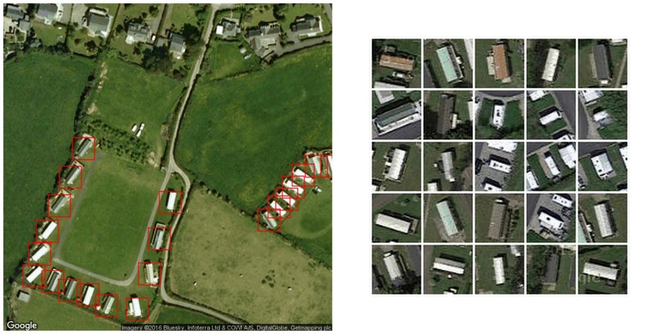
However, in all but OpenStreetMap, the precision was insufficient, often referring to the park entrance or location on a nearby road. Consequently, only the list extracted from OpenStreetMap was used to build a sample of 596 images of UK caravan parks. A further 599 images not containing caravan parks were randomly selected from Google Maps to make the final data for analysis. Examples of caravan park images can be seen in Figures 1a and 1b.
Figure 1a: Examples of used images of caravan parks (location 1)

Source: Google
Download this image Figure 1a: Examples of used images of caravan parks (location 1)
.png (291.2 kB)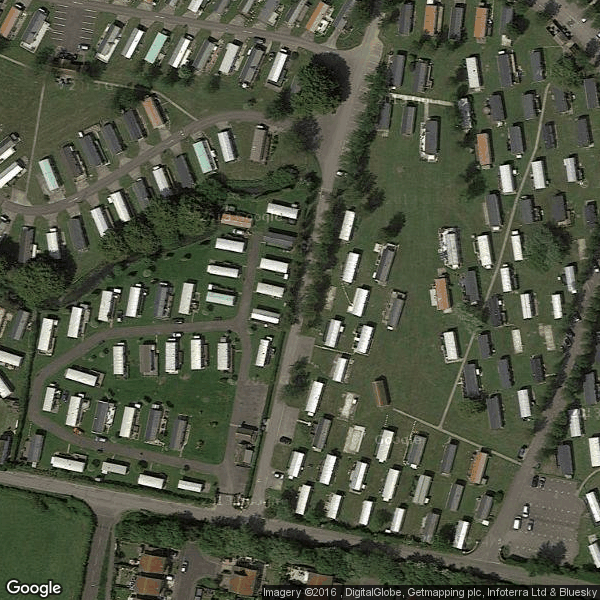
Figure 1b: Examples of used images of caravan parks (location 2)
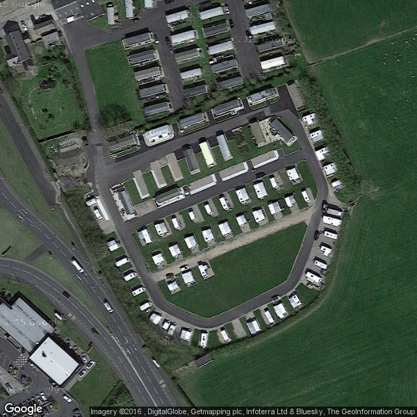
Source: Google
Download this image Figure 1b: Examples of used images of caravan parks (location 2)
.png (281.4 kB)
Pre-processing
The image data were downloaded in RGB (red, green, blue) format. RGB represents an image as a three-dimensional matrix where the values relate to the level of saturation for the three colour channels comprising each pixel (with 255 available levels)2. See Figure 2 for a visual representation of this.
To develop and assess any classification algorithm to detect images containing particular features such as caravans, it is necessary to have accurate labels distinguishing the positive and negative cases. The labels act as the dependent variable in subsequent models, while the RGB saturation values and other spectral measurements where available, comprise the explanatory variables. Image classification works by comparing the patterns of these measurements within the images.
Figure 2: Matrix representation of RGB (red, green, blue) image
Source: mathworks.com
Download this image Figure 2: Matrix representation of RGB (red, green, blue) image
.gif (5.1 kB)
As part of the explanatory variable analysis, the RGB profiles of the images were examined. For each colour channel, a histogram of pixel saturation was constructed by extracting the count of pixels with each level of saturation, as shown in Figure 3. The obtained functions tend to have irregular data points requiring a smoothing process before turning to machine learning. A linear kernel smoothing was applied to each histogram, that is, for each point the neighbouring values were averaged using weights decreasing by the distance from the treated point. The RGB profiles result in over 700 explanatory variables (255 possible levels of saturation across three colour channels).
Figure 3: The difference in RGB (red, green, blue) histograms between images containing caravans and other images

Notes:
- Notice the heavy right tails in the caravan images reflecting the fact that caravans tend to have a white roof.
Download this image Figure 3: The difference in RGB (red, green, blue) histograms between images containing caravans and other images
.png (55.7 kB) .csv (56.2 kB)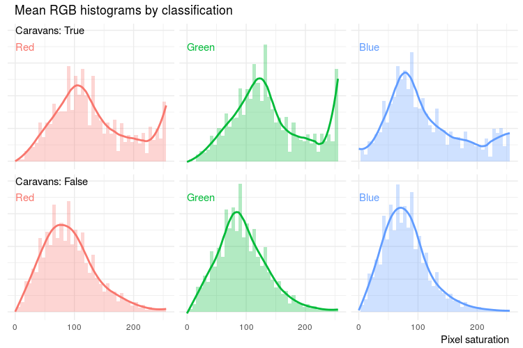
Methods
The aim of a classification process is to build an algorithm to automatically provide a class label based on some explanatory variables. Typically, image data are analysed using machine learning algorithms, which are trained based on the saturation values in available colour channels of the images. The learning can be either supervised or unsupervised depending on the purpose: in supervised learning, the ground truth (for example, class labels) is available for training, while the unsupervised learning attempts to infer hidden structure from unlabelled data. The results of the classification can then be used in a variety of ways from a simple prediction, such as the log odds of a class membership, to combining resulting likelihood-scores in more complex analysis.
Deep learning using convolutional neural networks is considered the cutting-edge algorithm in image recognition. This analysis compared neural networks with five other supervised classification algorithms3. As the most accurate, the neural network was further developed and combined with clustering techniques to provide the final output – a list of caravan sites where the detected image information disagreed with the AddressBase record.
Step 1: Full image classification
The data were split into a training set and test set, used to build and assess the models respectively. Analysis at this stage focused on finding a method that could classify the 1,195 labelled images into caravan parks and non-caravan parks. As an aerial photograph of a caravan park doesn't have a fixed natural orientation, it was possible to extend the size of the training set by transformations like rotation, reflection and translation. Zoom and resolution adjustments were applied to maximise classification performance.
Step 2: Improving performance using smaller image patches
A second dataset was derived by extracting individual caravans and their corresponding GPS position from 60 images. The small image patches were augmented using rotation and flip. Figure 4 shows examples of images in the transformed dataset. After adding the same number of images that did not contain caravans, the final dataset contained 45,000 images. These were split into test and training sets and further split into training and validation sets when necessary.
Figure 4: Examples of images in the second dataset - individual caravans
Source: Google, Office for National Statistics
Download this image Figure 4: Examples of images in the second dataset - individual caravans
.jpg (209.2 kB)
Step 3:Applying clustering to the output classifications
The classification output gives a score to each small image patch, therefore indicating likely locations of single caravans. For the purpose of this study, caravans within a small distance were grouped together and groups larger than 20 exported as a potential caravan park. These thresholds might require further optimisation.
Results
Supervised classification on the RGB profiles
Of the six supervised classification methods applied to both whole image as well as smaller image patches data, the best validation scores were achieved by Logistic Regression, Support Vector Machine and Random Forest on the full smooth RGB profile (73%, 72% and 71% correct classifications respectively). Random Forest achieved similar accuracy using the reduced variable set, with almost 70% correctly classified (see detailed output in Appendix 1)
Neural network classification of individual caravans
Details of the neural network architecture used can be found in Appendix 1.
An accuracy of 97% was achieved in identifying individual caravans within the second dataset of smaller image patches. This trained classifier for smaller image patches was then extended to the larger images of caravan parks in two different ways. The first one was through the neural network design by adding and training additional layers. The performance of this classifier on the whole images dropped down to 70%, which is comparable with the other machine learning algorithms mentioned previously.
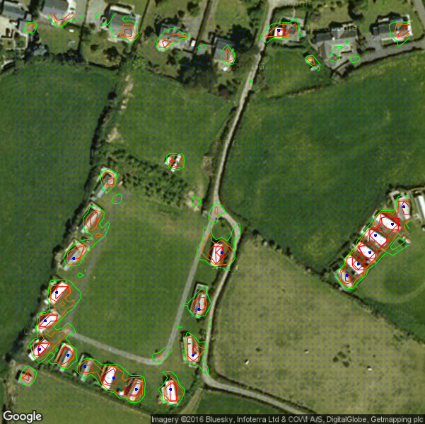
The second way requires outputting the classification score for each single image patch and post-processing (see Step 3: Applying clustering to the output classifications). The output or “classification score” can be interpreted as a heat-map of likelihood that a given spot in an image contains a caravan, see Figure 5.
Figure 5: Output heat-maps indicating likely locations of single caravans
Source: Google, Office for National Statistics
Notes:
- The colour changes from green to red as the likelihood grows.
- The blue dots represent locations classified by the algorithm as containing a caravan.
Download this image Figure 5: Output heat-maps indicating likely locations of single caravans
.png (630.8 kB)
Comparing the output against the AddressBase
From the heat-maps we extracted co-ordinates of sites likely to contain a caravan. To account for false positives, only locations with many potential caravans in close proximity were retained. This provided a list of caravan parks that could be compared with the AddressBase records of caravan parks.
Part of the area of Cornwall was processed and as a result about 70 locations (holding more than 1,500 caravans between them) were identified where fewer records were found in the AddressBase; these locations may, for example, contain holiday caravans.
Further applications – tract housing
Tract housing development is very common in the UK and often identifiable in aerial photography. Knowledge of tract housing has potential uses for imputation of non-response and quality control of house size-related questions4 in social surveys or the census. The extended neural network infrastructure built for caravan recognition was adapted to look for similar houses. In this case, the classification algorithm estimates similarity between a specific house and the neighbouring properties. The output of the algorithm in this case can be visualised as a heat-map of similarity of each patch to the central one, see Figure 6. In this case, we were not able to evaluate performance of this algorithm because no ground truth data were available at the time of analysis.
Figure 6: Output heat-maps indicating similar houses

Source: Google, Office for National Statistics
Notes:
- The colour changes from green to red as the similarity grows.
Download this image Figure 6: Output heat-maps indicating similar houses
.png (430.0 kB)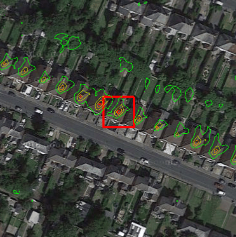
Notes for Caravan recognition pilot study
- It may be possible to purchase better quality commercial images for future work.
- For example, a 300-by-300-pixel image will have 90,000 values on the saturation scale of 0 to 255.
- These algorithms were Logistic Regression, Random Forest, Quadratic Discriminant Analysis, Gaussian Naïve Bayes, and Linear Support Vector Machine.
- For example, number of rooms, number of bedrooms.
4. Conclusion and future directions
This article is the result of rapid learning and initial experiences in handling and analysing aerial imagery data, where the focus has been on alternative data and methods to support address intelligence and quality of the AddressBase. This will be essential to the success of the 2021 Census. In particular, knowing the location and characteristics of unusual properties such as caravan homes is required for sending out internet access codes and for following up households that have delayed in completing their forms.
Aerial images were taken from Google maps and a neural network algorithm trained to identify single caravan homes with 97% accuracy. It is acknowledged that a 3% error rate leads to a large number of false positives over a large area (such as England and Wales), so results for single caravans were combined to help identify caravan parks containing clusters of caravans. The results have highlighted deficiencies in the number of caravans identified in AddressBase.
While several locations with missing or under-counted caravan parks have been identified and passed on to the Address Register Team, many more were considerably off-target. In particular, the amount of false positive cases over larger areas is of concern.
Opportunities for further improving classification performance are to:
improve quality of training and test datasets (for example, by including more images prone to misclassification – false positives from previous sprints)
include additional image channels (for example, Digital Terrain Model (DTM) and Digital Surface Model (DSM) from LIDAR data)
use published pre-trained neural networks for image features extraction (possibly as lower layers of the neural network design)
speed up the training process by taking more advantages of the cloud and parallelised computing systems including Graphical Processing Units (GPU)
5. References and other useful links
Official statistics context
United Nations Statistics Division: Task Team on Satellite Imagery and Geo-Spatial Data (2015)
Australian Bureau of Statistics (Methodology Advisory Committee): Methodological Approaches for Utilising Satellite Imagery to Estimate Official Crop Area Statistics (2014)
United States Agricultural Statistics Service: Reported Uses of CropScape and the National Cropland Data Layer Program (2013)
Indian Institute of Science: Relevance of Hyperspectral Data for Sustainable Management of Natural Resources (2006)
Deep learning references
Richards JA and Jia X (2013), Remote Sensing Digital Image Analysis
Goswami AK, Gakhar S and Kaur H (2014), Automatic Object Recognition from Satellite Images using Artificial Neural Network (2014)
Mokhtarzade M and Valadan Zoej MJ (2006), Road detection from high-resolution satellite images using artificial neural networks
Kavukcuoglu K, Ranzato MA and LeCun Y (2014), Classify a satellite image using a convolutional neural network (part of web resources compiled by Roy Hyunjin Han)
Harvey RL, DiCaprio PN and Heinemann KG (1991), A Neural Network Architecture for General Image Recognition
Logical methods of object recognition on satellite images using spatial constraints
Ke Y and others (2009), A Rapid Object Detection Method for Satellite Image with Large Size
Erus G and Loménie N (2005), Automatic Learning of Structural Models of Cartographic Objects
6. Appendix 1
Overview of the used classification methods
The task at hand was to automatically assign labels (“is it a caravan or not?”) to images. This is called supervised binary classification in the machine learning context and various methods are available. This section provides a summary explanation of the techniques used. Note that the available explanatory variables (in this case RGB (red, green, blue) values) are referred to as features and the dependant labels as classes.
Logistic Regression
The log odds of the binary outcome are modelled as a linear combination of the features. The parameters and weights of each feature are obtained, which can be used to explore the strength of each feature. In a model with a large number of features, it is desirable to introduce regularisation to prevent over-fitting.
Over-fitting occurs when a model describes the random error in data and not the underlying relationships and means that the model does not work well on new, or unseen, data. An L2 penalty was used for regularisation, that is, a sum of squares of the parameter values was added to the total cost (negative log likelihood) during optimisation.
Random Forest
Decision trees are tree-like charts or diagrams used to represent a sequence of decisions. Each node leads to splitting the data into subsets based on one feature rule. Ideally, the terminal nodes (those at the end of the branches) would then hold one class label (that is, whether the picture is a caravan or not). Algorithms for constructing decision trees usually work top-down, by choosing a feature at each step that best splits the set of items, until a pre-set stopping rule is met (we used the entropy criterion). Random Forest is a group of decision trees, trained on different subsets of data, to correct for over-fitting that can come from using a single decision tree.
Naïve Bayes, LDA and QDA
Gaussian Naïve Bayes, Linear Discriminant Analysis (LDA) and Quadratic Discriminant Analysis (QDA) are all classifiers that create a conditional probability model so that the probability of class membership is calculated based on the feature values. In the LDA and QDA, class membership is assumed to have multivariate normal distribution, where LDA assumes equal covariates across classes, while QDA optimises class-specific covariates. Gaussian Naïve Bayes treats the conditional density as a product of univariate normal distributions.
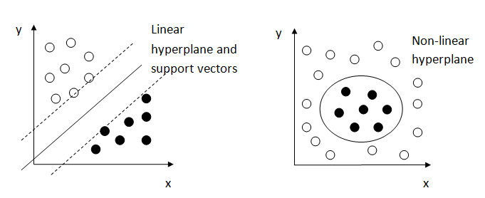
Support Vector Machine (SVM)
The features are viewed as co-ordinates in high-dimensional space and the SVM aims to separate points belonging to different classes by a hyperplane. The weights are optimised by finding a hyperplane with smallest cost of misclassification and largest margin between the hyperplane and the data points (where the closest ones are called support vectors). Often the linear separation is not optimal and a kernel trick is used to transform data points before a linear hyperplane is fitted. In Figure 7, the example on the left-hand side illustrates a linear separation, while the example on the right-hand side shows a hyperplane with a non-linear kernel.
Figure 7: Graphical depiction of Support Vector Machine
Source: Office for National Statistics, Working paper series 1
Download this image Figure 7: Graphical depiction of Support Vector Machine
.png (15.8 kB)
Evaluation of binary classifiers
To evaluate a classifier, we compare its output to the ground truth and construct a confusion matrix. The fields in the confusion matrix correspond to the number of data points falling in each of the four possible categories:
- TP – true positive
- FP – false positive (Type I error)
- TN – true negative (correct rejection)
- FN – false negative (Type II error)
Table 1 provides an example of a confusion matrix.
Table 1: Confusion matrix example
| Ground truth (by eye) | ||||
|---|---|---|---|---|
| Caravan image | No caravan | |||
| Classifier | Caravan image | TP | FP | |
| No caravan | FN | TN | ||
Download this table Table 1: Confusion matrix example
.xls (34.3 kB)There are several metrics that give a single number to evaluate the classifiers described previously. Their usage depends on the type of data, that is, whether the classes are balanced (that is, there are an equal number of caravan and non-caravan pictures) or whether one type of error is considered more serious. The two most commonly used are accuracy and F1-score.
Accuracy quantifies the proportion of correctly classified data points, while the F1-score is the harmonic mean of recall (proportion of correctly classified cases out of all true positives) and precision (proportion of correctly classified cases out of all classified as positive).
Accuracy is calculated using the following equation:
F1-score is calculated using the following equation:
Both these measures take values between 0 and 1 with higher values meaning better classifier.
K-fold cross-validation
Cross-validation is a technique to evaluate models using the training data divided into k mutually exclusive subsets. In each fold, a single sub-sample is retained as the validation data for testing the model and the remaining k-1 sub-samples are used for model training. The purpose of cross-validation is to identify the best model (or its hyper-parameters) and to get an accurate impression of how well the model performs and generalises to unseen data.
We used cross-validation to optimise hyper-parameters of some of the models mentioned previously, for example, penalty choice l1/l2 for the logistic regression and SVM parameters.
RGB profiles output summary
Here we present a summary of the classification results applied during RGB profile analysis described in Section 3 =.
The smooth RGB profiles were used as input for several classification algorithms. Dimensionality reduction by principal component analysis (PCA) was applied to the smoothed data. PCA is used in datasets containing a large number of features to reduce the number to a few, linear combinations of the data. Often, its operation can be thought of as revealing the underlying factors in a way that best explains the variance in the data. Undertaking PCA on the data resulted in 43 components that explained 95% of the variation.
Table 2 contains performance measures for each method when applied to the (full) smooth RGB profiles as well as to the set of principal components (explaining 95% variability).
Table 2: Summary of performance of supervised classification algorithms on RGB (red, green, blue) profiles
| Method | Dimensionality reduction | Accuracy (%) | F1-score (%) |
|---|---|---|---|
| Logistic Regression (l2 penalty) | None | 72.6 | 71.6 |
| PCA | 65.8 | 64.1 | |
| Random Forest (entropy criterion) | None | 71.5 | 70.3 |
| PCA | 69.6 | 68.1 | |
| Quadratic Discriminant Analysis (collinearity warning) | None | 51.3 | 15.9 |
| PCA | 68.8 | 64.6 | |
| Gaussian Naive Bayes | None | 63.3 | 56.6 |
| PCA | 64.5 | 57.2 | |
| Linear Support Vector Machine (l1 penalty) | None | 72.1 | 71.4 |
| PCA | 65.7 | 64.2 |
Download this table Table 2: Summary of performance of supervised classification algorithms on RGB (red, green, blue) profiles
.xls (35.3 kB)Neural Network design
The basic idea behind a neural network is to simulate lots of densely interconnected brain cells inside a computer so that it can learn things, recognise patterns and make decisions in a humanlike way. Neural network is a machine learning method based on learning high-level representations of data by using multiple processing layers composed of multiple non-linear transformations. Designing and training of a neural network is a difficult and resource expensive task.
A commonly used design in the area of image recognition is convolution network based on the LeNet-5 architecture. We started with implementing this model in Python using libraries Theano (with Lasagne) and Tensorflow (they both use parallel computing and the C programming language under the Python interface).
Figure 8: Graphical depiction of LeNet architecture.

Source: deeplearning.net
Download this image Figure 8: Graphical depiction of LeNet architecture.
.png (49.8 kB)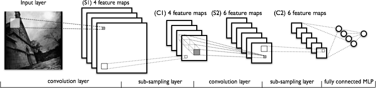
A summary of layers in the used neural network can be found in Table 3. It is based on the LeNet-5 architecture. During training, we used mini batches (that is, smaller subsets of data were used in one step) and applied 50% dropout to the fully connected layer (to prevent overfitting). We experimented with neural network architecture as well as parameters of the previously mentioned design (for example, filter sizes, number of channels), but no significant improvement over this basic design was achieved.
Table 3: Neural Network Design
| Layer | Description | Size for | |
| SMALLER IMAGES | BIGGER IMAGES | ||
| Input | 24x24 nodes in 3 channels | 300x300 nodes in 3 channels | |
| Convolution | 5x5 filter, bias and rectified linear non-linearity | 20x20 nodes in 32 channels | 296x296 nodes in 32 channels |
| Sub-sampling | max-pooling over 2×2 window | 10x10 nodes in 32 channels | 148x148 nodes in 32 channels |
| Convolution | 5x5 filter, bias and rectified linear non-linearity | 6x6 nodes in 32 channels | 144x144 nodes in 32 channels |
| Sub-sampling | max-pooling over 2×2 window | 3x3 nodes in 32 channels | 72x72 nodes in 32 channels |
| Fully connected/Convolution | 3x3 filter, bias and rectified linear non-linearity | 1 node in 32 channels | 70x70 nodes in 32 channels |
| Dropout | 50% dropout during training | 1 node in 256 channels | 70x70 nodes in 256 channels |
| Output | soft-max non-linearity | 1 node in 1 channel | 70x70 nodes in 1 channel |
Download this table Table 3: Neural Network Design
.xls (37.4 kB)Hardware specifications
The work was undertaken in the Innovation Lab (ONS private cloud environment) on a virtual machine with four cores and 40GB RAM. Further information about the Innovation Lab is available in ONS methodology working paper series number 1 – ONS Innovation Laboratories (PDF, 1.2MB).
Many machine learning algorithms used (including neural nets) are parallelisable and so possible use of GPU was explored. Commonly-used hardware for this task is NVIDIA graphics card with higher than 3.5 computing capabilities. At the time of implementation, we had available NVIDIA card of 3.0 computing capabilities and Radeon AMD graphics card. They don’t satisfy minimal requirements of Tensorflow, so we experimented with using Theano (through Cuda or OpenCL) instead.
Back to table of contents