A guide to interpreting monthly gross domestic product

One of the statistical challenges highlighted in the Independent Review of UK Economic Statistics (PDF 5.13MB) (Sir Charles Bean, 2016), relates to “the scope for improving early estimates of gross domestic product (GDP) through the use of administrative data, including by making greater use of information from the expenditure and income measures”. In response, we have now moved to the new gross domestic product (GDP) publication model. There is now a higher data content in the new first quarterly estimate of GDP, which is expected to improve the trade-off between the timeliness and accuracy of early estimates, resulting in fewer revisions.

As part of this work we have sped up the publication of the Index of Services (IoS) by over two weeks, which means that the Index of Production (IoP), construction output and IoS are now all published on the same date, and combined these make up 99.3% of gross value added (GVA) in 2016 weights. This means that the UK has now become one of just a handful of countries producing official estimates of monthly GDP, providing users of economic statistics a more timely and coherent picture of the UK economy. Detailed data will continue to be published in the IoP, construction output and IoS monthly bulletins.

In the output approach to measuring GDP, we use GVA as a proxy for GDP and therefore the almost complete coverage of monthly GVA leads to the production of new statistics including a rolling three-month-on-three-month estimate of GDP and an estimate of GDP in the latest month. This new publication will give the high-level details of the GDP movements as described in the Monthly GDP; more information faster blog by James Scruton on 4 July 2018. Outside of the sphere of official statistics, the UK has a longer history in this field with the National Institute of Economic and Social Research (NIESR) producing estimates, primarily based on our data, since April 1998. Our latest developments advance work in this field to provide a better understanding of the short-term evolution of the economy. Further details on the NIESR data and methods can be found on their website.

This article serves as a guide to interpreting estimates of monthly GDP. It outlines the difference between GVA and GDP; provides some information about the possible volatility in the monthly GDP estimates; gives an indication of what are the causes of this volatility; and explains how to interpret the monthly GDP estimates. For these reasons, our lead indicator will be the three-month-on-three-month GDP movements, with the individual months that make up this picture provided alongside for completeness.

Ideally the analysis contained in this article would be produced using the “first published” estimates of monthly GDP. However, these are not available historically so we can only use the current position, which will differ slightly from those published in real time. These estimates should be less volatile than when first published because the quarterly and annual data that are formed from these monthly estimates have been through the annual supply and use balancing process. Going forwards, we plan to produce a real-time monthly GDP database during the second half of 2018, including the underlying components of GDP, which will enable full revisions analyses in the future.

In the national accounts, gross domestic product (GDP) is measured by the output, income and expenditure approaches. In the output approach, we use gross value added (GVA) as a proxy for GDP. GVA is the value of an industry’s outputs less the value of intermediate inputs used in the production process. On a quarterly basis, GVA is aligned to be within plus or minus 0.2 percentage points of quarterly GDP in supply-use balanced years (up to and including 2016 in the latest estimates on 10 July 2018). As such, the path of quarterly GVA is similar to the published quarterly GDP figures as shown in Figure 1, meaning that GVA is a good proxy for GDP, and we will use the terminology of GDP within the statistical releases for ease of communication. In more recent periods, GVA and GDP are not fully aligned, except in the very latest two quarters where balanced GDP and GVA will be exactly equal and so the growth rates of GDP and GVA will only ever be guaranteed to be equal when comparing the latest quarter with the previous quarter.

The alignment process that is performed for the quarters does not happen within the individual months of a quarter, so it is possible that monthly GVA and a true estimate of monthly GDP would deviate by slightly more. However, monthly GVA will be a good approximation for monthly GDP and present a picture of UK economic performance that is entirely consistent with the latest quarterly GDP estimates.

When using the output approach to measuring gross domestic product (GDP) we are actually estimating the contribution of each industry or producer by using gross value added (GVA) at basic prices – or put simply the value of a unit’s outputs less the value of inputs used in the production process to produce the outputs. The basic price is the amount that the producer receives for a unit of a good or service that is produced. As such, it includes any subsidies that are received on products but excludes any taxes that are payable on those products.

The link between GVA and GDP is:

GVA at basic prices

plus taxes on products

less subsidies on products

equals GDP at market prices (or headline GDP).

Growth rates of GDP and GVA can differ because of the differences between market prices and basic prices. Given that the prices used are different it is not surprising that at times the growth rates will also differ.

Because of the higher data content in output, the growth rates of average GDP in both the current and immediately preceding quarter are set equal to the growth rates of output GVA via balancing adjustments to production, income and expenditure components of GDP. Prior to the latest two quarters GDP and GVA growth rates may differ.

Monthly gross domestic product (GDP) data have been published back to 1997, giving over 21 full years of monthly figures. This article looks at the data from January 1997 to December 2017. Figure 2 shows the level of monthly GDP and by construct the underlying profile is the same. However, it is notable that there is a little more noise in the monthly profile, with the timings of the special events of 2002 and 2012 (and the recession of 2008 to 2009) standing out in particular. 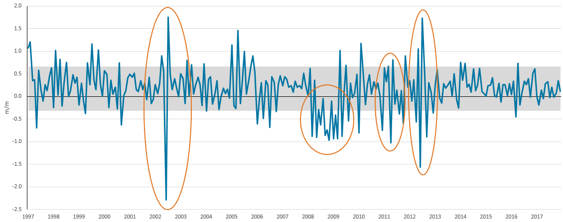This reflects that monthly GDP estimates are inherently more volatile than the quarterly ones.

This increase in volatility in the monthly estimates can be seen more clearly in Figure 3. Shading has been added to show one standard deviation of monthly GDP movements, approximately between negative 0.3% and positive 0.7% growth. Two things are striking about Figure 3 – the large number of months that have seen zero or negative growth and how certain periods in economic history have displayed a much more volatile monthly GDP path than might be expected from the already published quarterly data.

Figure 3: Monthly GDP growth rates from 1997 to 2017, UK

Source: Office for National Statistics

Download this image Figure 3: Monthly GDP growth rates from 1997 to 2017, UK

.png (79.2 kB)

Firstly, we look at the months that have negative growth, as these would tend to get more attention on publication day. Between Quarter 1 (Jan to Mar) 1997 and Quarter 4 (Oct to Dec) 2017 there have been seven quarters of negative growth – that is, there have been fewer than 1 in 10 quarters that have seen a fall in output over this period. Yet within the same timespan we have had 60 negative growth months out of 252, which is nearly one in every four months. Even if we narrow the timespan to be only the quarters after the last negative GDP quarter (Quarter 4 2012), we have still seen seven months of negative growth and a further 12 months with zero growth out of 60 months (12% of months are negative and 32% of all months have recorded negative or zero growth). The clear message here is that the monthly GDP will, by definition, be more volatile than the quarterly data where individual monthly movements get “smoothed” out more.

Secondly, Figure 3 also shows periods in economic history where monthly GDP has deviated from the expected range by more than one standard deviation. There are four periods in the data range where monthly GDP has had a much more volatile path than might be expected, while there was increased volatility through 2005 caused by the challenges of profiling a monthly path through some of our quarterly services data.

Four periods of volatile GDP

June to July 2002: The Queen’s golden jubilee resulted in two bank holidays in early June, the first being delayed from May and the second being an extra one. This extra bank holiday contributed to a fall in monthly GDP of 2.3% on current estimates. GDP then recovered in July as expected after the one-off special event, with a rise of 1.8%.

2008 to 2009: The recession caused by a financial crisis, with GDP falling 6.3% peak to trough. The monthly movements within this period are not very volatile as all monthly growths fall within quite a narrow range, but the widespread effects of the credit crunch are plain to see.

December 2010 to April 2011: A range of special events dominated the monthly movements including heavy snowfall causing disruption in December 2010 and then, in early 2011, there was an additional bank holiday because of the wedding of the Duke and Duchess of Cambridge. This extra bank holiday fell soon after Easter and many people took the opportunity for an extended break. There was also record warm weather; it was the warmest April in over 100 years.

June to September 2012: June 2012 saw the Queen’s diamond jubilee with two bank holidays in early June, the first being delayed from May, and the second being an extra bank holiday. The London 2012 Olympic and Paralympic games took place between 27 July and 9 September, bringing increased tourism and ticket sales to the UK.

Other than the impacts of the financial crisis of 2008 to 2009, these episodes highlight the effects of lost and/or displaced activity from one-off factors, which has a more pronounced effect on monthly GDP estimates. One of the reasons is that there is less scope for activity to be displaced within a month than it can be within a quarter. While these temporary effects may be smoothed out within a quarter, there is an increased likelihood of this being reflected in a more volatile monthly path. The effects can also be larger in specific areas of the economy – for instance, the nature of construction activity is that this will typically see much more volatile movements during periods of adverse weather.

Services is the largest contributor to gross domestic product (GDP), in terms of its weight at 79.6% of the economy. It is therefore not a surprise that when the service sector experiences volatile growth, so GDP as a whole is likely to experience volatile growth.

Figure 4 shows the contributions to growth during the years 2011 and 2012, as several special events hit the UK economy in this period. In most months, all sectors move in a similar manner, and it is the weight of services that provides the largest contribution to growth. This is usually the case when there is an extra bank holiday or a weather event, which tend to impact across all sectors. For instance, output in all sectors fell because of the snowfall of December 2010, all sectors fell with the extended period of holidays in April 2011, and all sectors fell sharply in June 2012 with the jubilee events. It also reinforces how the monthly path can be particularly volatile in such periods, as businesses look to recover this output in the following month. This is clearly seen in January 2011, May 2011, May 2012 and July 2012. It is worth noting that despite this period being particularly volatile because of several special events, this period of 27 months saw 10 months with negative GDP growth, which is only a slightly higher proportion than the average seen since 1997.

Against the backdrop of special events in this period, there are still months where the individual sectors do not all move in the same direction, as might be expected given the varying nature of the sectors. In February 2011, while services increased there was a large decrease in production output. This was caused by large falls in both mining and quarrying (owing to unseasonal maintenance work and slow-downs in output), and electricity, gas and water supply (because of very mild temperatures). In January 2012, a large fall in construction, following a strong December 2011 figure, partially offset the strong services growth. The Index of Production can be volatile because of non-manufacturing components, for example, mining and quarrying because of unseasonal maintenance or disruption to the extraction and transportation of oil and/or gas. Electricity, gas and water supply can be affected by unseasonably warm or cold weather. Construction output can also be volatile because of the nature of the construction industry with the completion of projects as well as impacts from the weather.

In summary, there can be considerable volatility from month to month in the GDP figures, and this is usually driven by the services sector because of its large weight in output GDP. Special events play a role in some of the monthly volatility, such as extra bank holidays, the Olympics in 2012 or extreme weather events. Usually the effect of this monthly volatility is dampened by the time quarterly figures are compiled, unless the event is in the first or last month of the quarter when there may potentially be some displacement into other quarters.

Monthly GDP data is a new and informative product on the state of the economy with a high data content for output. However, users should still avoid reading too much into a single month’s figure, especially if there are particular circumstances that might make that month more volatile than usual. Early forecasts for the quarter ahead should therefore not be drawn from just the first month of that quarter when it is published. We will lead with the three-month-on-three-month figure for GDP, as this smooths out some of the volatility and presents a better picture of the state of the economy.

Generally speaking, the rolling three-month-on-three-month GDP estimates are less volatile than the monthly series and track within a range seen by the existing quarterly GDP estimates. However, the impacts of particularly large monthly movements can still be seen in some of the three-month-on-three-month movements (Figure 5). These show up where the blue lines either side of the yellow dots of quarterly GDP are a long way apart, with the main differences in 2002 when there was the Queen’s golden jubilee, and a further one in 2011 for the snowfall in December, the record-breaking warm weather of April 2012 and the wedding of the Duke and Duchess of Cambridge in the same month.

The 2002 golden jubilee is an example of how a volatile monthly GDP figure can still contribute to the three-month-on-three-month figure being a potentially misleading indicator of the underlying state of the economy. If we had published this three-month-on-three-month GDP movement at the time, this special event would have led to a slowdown from the 1.2% three-month-on-three-month growth published in May 2002 to 0.7% in the three months to June 2002.

As the three-month-on-three-month picture worked through this volatile monthly path, including the recovery in July, as well as other unrelated movements in the months ahead of the jubilee, three-month-on-three-month growth dipped to negative 0.3% in August before recovering to positive 0.8% in September 2002 for the next quarterly estimate. The quarterly GDP movements were positive 0.7% for Quarter 2 (Apr to June) 2002 and positive 0.8% for Quarter 3 (July to Sept) 2002. However, using the rolling three-month-on-three-month estimates, economic growth ranged from positive 1.2% in May 2012 to negative 0.3% in August 2012, a very different picture from that painted by just the quarterly data.

Despite these rare monthly impacts on three-month-on-three-month growth, broadly speaking the three-monthly movements lessen the volatility seen in the month-on-month GDP growth, and therefore are a better indicator of the underlying direction and strength in the economy. In our publications we will draw attention to any particularly large or unusual monthly movements to put them into context and avoid users drawing the wrong conclusion from a single point of monthly data. We will also clearly explain when a single monthly movement is having a large influence on the three-month-on-three-month GDP estimate and how this monthly movement will cause the three-month-on-three-month movement to fluctuate.

The UK has now become one of the first countries to produce official estimates of monthly gross domestic product (GDP). This is a much-anticipated product that will give a more complete picture of the economy earlier on in the months following the quarter as well as becoming a leading-edge indicator. The first estimate of quarterly GDP will also have a much higher data content than the previous preliminary estimate, so a slightly later publication of the first estimate of GDP has the potential to lead to a reduction in the magnitude of later revisions. We are also committed to reviewing continuously how we can improve the quality of early estimates of GDP as part of our wider transformation programme.

Monthly GDP data is much more prone to volatility than quarterly GDP data with almost one month in every four over the last 21 years showing negative GDP growth. Interpretation of these new outputs is therefore key and we have developed a new monthly GDP publication to focus on presenting the three-month-on-three-month GDP estimates as well as the monthly GDP estimates. We have developed a new bulletin to make monthly GDP more accessible to the wider public. The new style publication has been designed to be much more of a visual piece with headline graphics and will be much shorter in length than existing bulletins. It has been developed in response to user feedback for a more engaging publication that is more consistent with the time spent by visitors to our website. We welcome feedback on the outputs being published and the way in which these estimates are presented.