Effects of taxes and benefits on UK household income: financial year ending 2015

In the financial year ending 2015 (2014/15), the average income of the richest fifth of UK households before taxes and benefits was £83,800, 14 times greater than that of the poorest fifth who had an average income of £6,100 per year.

After taking into account taxes and benefits the ratio between the average incomes of the top and the bottom fifth of households (£62,500 and £16,500 respectively) is reduced to 4 to 1.

The richest fifth of households paid £29,800 in taxes (direct and indirect) compared with £5,200 for the poorest fifth.

In 2014/15, 50.8% of all households received more in benefits (including benefits in kind) than they paid in taxes, equivalent to 13.6 million households. This continues the downward trend seen since 2010/11 (53.5%), but remains above the proportion seen before the economic downturn.

On average, households whose head was between 25 and 64 paid more in taxes than they received in benefits (including in-kind benefits) in 2014/15, whilst the reverse was true for those aged 65 and over.

Analysis on changes in median household disposable income and other related measures, which used to form part of this report, were published earlier this year in “Household Disposable Income and Inequality, financial year ending 2015”. This new bulletin was introduced in response to demand for more timely information on certain headline indicators. The current report provides more in-depth analysis, focusing on the overall impact of the tax and benefits system on household incomes for different groups.

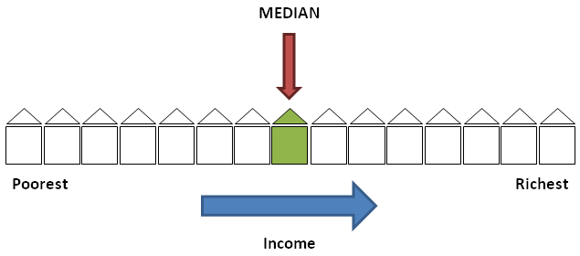
Figure 1: Stages in the redistribution of income

Source: Office for National Statistics

Download this image Figure 1: Stages in the redistribution of income

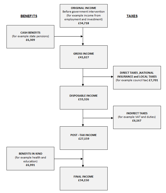
.PNG (21.7 kB) .doc (41.5 kB)

This release looks at how taxes and benefits affect the distribution of income in the UK and breaks this process into 5 stages. These are summarised in Figure 1 and below:

1. Household members begin with income from employment, private pensions, investments and from other non-government sources. This is referred to as “original income”.

2. Households then receive income from cash benefits. The sum of cash benefits and original income is referred to as “gross income”.

3. Households then pay direct taxes. Gross income minus direct taxes is referred to as “disposable income”.

4. Indirect taxes are then paid via expenditure. Disposable income minus indirect taxes is referred to as “post-tax income”.

5. Households finally receive a benefit from services (benefits in kind). Benefits in kind plus post-tax income is referred to as “final income”.

The overall impact of taxes and benefits are that they lead to income being shared more equally between households. In 2014/15, before taxes and benefits, the richest fifth (those in the top income quintile group) had an average original income of £83,800 per year, compared with £6,100 for the poorest fifth – a ratio of 14 to 1 (Figure 2).

After cash benefits and direct taxes, the richest fifth of households had average incomes that were around 5 and a half times that of the poorest fifth (£67,000 and £12,300 per year respectively).

After accounting for all taxes and benefits, including indirect taxes and benefits in kind, in 2014/15 the ratio of the income of the richest fifth of the population to the poorest fifth (£62,500 and £16,500 per year respectively), further reduced to less than 4 to 1.

These ratios are broadly similar to those in 2013/14, indicating that inequality of income has not changed substantially between the 2 years, according to these measures.

Impact of cash benefits

In contrast to original income, the amount received from cash benefits such as tax credits, Housing Benefit and Income Support tends to be higher for poorer households than for richer households. As a result, cash benefits act to reduce income inequality. In 2014/15, the highest amount of cash benefits was received by households in the second quintile group, £8,900 per year compared with £7,700 for households in the bottom group (Figure 3). This is largely because more retired households are located in the second quintile group compared with the bottom group and in this analysis the State Pension is classified as a cash benefit.

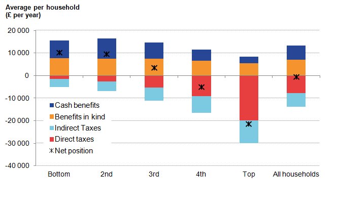
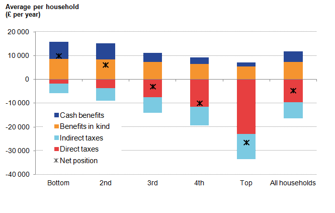
Figure 3: Summary of the effects of taxes and benefits by quintile groups, ALL households, financial year ending 2015, UK

Source: Office for National Statistics

Download this image Figure 3: Summary of the effects of taxes and benefits by quintile groups, ALL households, financial year ending 2015, UK

.png (14.0 kB) .xls (11.2 kB)

Looking at individual cash benefits, in 2014/15, the average combined amount of contribution-based and income-based Jobseeker’s Allowance (JSA) received by the bottom 2 quintile groups decreased compared with 2013/14 (Effects of taxes and benefits dataset Table 2). This is largely due to fewer households receiving this benefit, consistent with a fall in unemployment between these years, as well as the ongoing implementation of the Universal Credit (UC) system which by April 2015 had been rolled out to 85,000 claimants¹.

Claimants of UC and JSA are subject to the Claimant Commitment which outlines specific actions that the recipient must carry out in order to receive benefits. This may also have affected the number of households in receipt of these benefits. JSA rates, along with other working age benefits, were increased by 1% in 2014/15, below the CPI rate of inflation. The phasing out of Incapacity Benefit, Severe Disablement Allowance and Income Support paid because of illness or disability and transfer of recipients to Employment and Support Allowance (ESA) has seen average amounts received from the former benefits fall in 2014/15, whilst average amounts received from ESA have risen, reflecting the increased number of claimants. The roll-out of Personal Independence Payment (PIP), which is replacing Disability Living Allowance (DLA) for adults aged under 65², also continued in 2014/15.

There was a 20.3% decrease in the amount of Child Benefit received by the richest fifth of households, due to fewer households in this part of the income distribution receiving this benefit. This is likely to be related to the High Income Benefit Charge, which came into effect in January 2013. From this date, those on higher incomes were liable to pay a charge equivalent to some or all of their child benefit entitlement, which may have resulted in some households electing to stop getting Child Benefit (“opt out”) rather than pay the charge.

Impact of direct taxes

Direct taxes (Income Tax, employees’ National Insurance contributions and Council Tax or Northern Ireland rates) also act to reduce inequality of income. Richer households pay both higher amounts of direct tax and a higher proportion of their income in direct taxes.

In 2014/15, on average, households paid £7,700 per year in direct taxes, equivalent to 18.8% of their gross income (Figure 4). The richest fifth of households paid, on average £19,800 per year, which corresponds to 22.8% of their gross income. The majority of this (16.3% of gross income) was paid in Income Tax. The average tax bill for the poorest fifth of households, by contrast was £1,500 per year, which is equivalent to 11.0% of their gross household income. Council Tax or Northern Ireland rates made up the largest proportion of direct taxes for this group, accounting for half of all direct taxes paid by them, 5.5% of their gross income on average.

The poorest fifth of households had the largest annual percentage increase in the average amount paid in Income Tax in 2014/15, increasing from £417 per year in 2013/14 (2014/15 prices) to £550 per year in 2014/15, equivalent to an increase of 32%. However, the average amount paid as a proportion of their gross income was largely unchanged (4.0% in 2014/15 compared with 3.2% in 2013/14). This reflects both an increase in employment and an increase in the average amount received in wages and salaries in this part of the distribution, which has masked the effect of the increase in the personal allowance (from £9,440 in 2013/14 to £10,000 in 2014/15).

Further analysis on the impact of cash benefits and direct taxes on disposable income can be found within the “Household Disposable Income and Inequality, financial year ending 2015” publication.

Impact of indirect taxes

The amount of indirect tax (such as Value Added Tax (VAT) and duties on alcohol and fuel) each household pays is determined by their expenditure rather than their income. The richest fifth of households paid just over 2 and a half times as much in indirect taxes as the poorest fifth (£10,000 and £3,700 per year, respectively). This reflects greater expenditure on goods and services subject to these taxes by higher income households. However, although richer households pay more in indirect taxes than poorer ones, they pay less as a proportion of their income (Figure 5). This means that indirect taxes increase inequality of income.

In 2014/15, the richest fifth of households paid 15.0% of their disposable income in indirect taxes, while the bottom fifth of households paid the equivalent of 29.7% of their disposable income. Across the board, VAT is the largest component of indirect taxes. Again, the proportion of disposable income that is spent on VAT is highest for the poorest fifth and lowest for the richest fifth.

Grouping households by their income is recognised as the standard approach to distributional analysis, as income provides a good indication of households’ material living standards, but it is also useful to group households according to their expenditure, particularly for examining indirect taxes, which are paid on expenditure rather than income. Some households, particularly those at the lower end of the income distribution, may have annual expenditure which exceeds their annual income. For these households, their expenditure is not being funded entirely from income. During periods of low income, these households may maintain their standard of living by funding their expenditure from savings or borrowing, thereby adjusting their lifetime consumption.

When expressed as a percentage of expenditure³, the proportion paid in indirect tax declines less sharply as income rises (Figure 6) compared with the level of indirect taxes paid as a proportion of household disposable income. The bottom fifth of households paid 20.1% of their expenditure in indirect taxes compared with 17.6% for the top fifth. These figures are broadly unchanged from the previous year.

After indirect taxes, the richest fifth had post-tax household incomes that were 6 and a half times those of the poorest fifth (£56,900 compared with £8,700 per year, respectively). This ratio is unchanged on 2013/14.

Impact of benefits in kind

This publication also considers the effect on household income of certain benefits received in kind. Benefits in kind are goods and services provided by the government to households that are either free at the time of use or at subsidised prices, such as education and health services. These goods and services can be assigned a monetary value based on the cost to the government which is then allocated as a benefit to individual households. The poorest fifth of households received the equivalent of £7,800 per year from all benefits in kind, compared with £5,500 received by the top fifth (Effects of taxes and benefits dataset Table 2). This is partly due to households towards the bottom of the income distribution having, on average, a larger number of children in state education.

Notes on Summary of the effects of taxes and benefits for all households

1. The number of people in the survey sample indicating they received Universal Credit (UC) was too small to allow it to be represented separately in this analysis. UC has therefore been classified under ‘other cash benefits’.
2. In England, Wales and Scotland.
3. Expenditure is calculated to be consistent with disposable income.
4. Throughout this release, 2014/15 refers to the financial year ending 2015 and similarly for other years in this format.

Overall, in 2014/15, 50.8% of all households received more in benefits (including in-kind benefits such as education) than they paid in taxes (direct and indirect) (Figure 7). This equates to 13.6 million households. This continues the downward trend seen since 2010/11 (53.5%) but remains above the proportions seen before the economic downturn.

The trend seen for non-retired households mirrors that for all households, except that lower percentages of non-retired households receive more in benefits than pay in taxes, 36.9% in 2014/15, down from a peak of 39.7% in 2010/11.

In contrast, in 2014/15, 88.7% of retired households received more in benefits than paid in taxes, reflecting the classification of the State Pension as a cash benefit in this analysis. A retired household is defined as a household where the income of retired household members accounts for the majority of the total household gross income². This figure is lower than its 2009/2010 peak of 92.4% but is broadly similar to the proportions seen before the downturn.

Notes on Households receiving more in benefits than paid in taxes

1. See background notes for definition of retired person.
2. Throughout this release, 2014/15 refers to the financial year ending 2015 and similarly for other years in this format.

There are a number of different ways in which inequality of household income can be presented and summarised. Perhaps the most widely used measure internationally is the Gini coefficient. Gini coefficients can vary between 0 and 100 and the lower the value, the more equally household income is distributed.

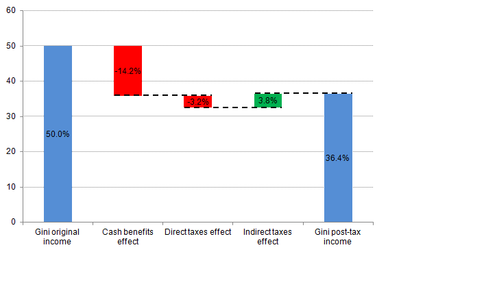
The extent to which cash benefits, direct taxes and indirect taxes together work to affect income inequality can be seen by comparing the Gini coefficients of original, gross, disposable and post-tax incomes (Effects of taxes and benefits dataset Table 10). Cash benefits have the largest impact on reducing income inequality, in 2014/15 reducing the Gini coefficient from 50.0% for original income to 35.8% for gross income (Figure 8). Direct taxes act to further reduce it, to 32.6% in 2014/15. However, indirect taxes have the opposite effect and in 2014/15 the Gini for post-tax income was 36.4%, meaning that overall, taxes have a negligible effect on income inequality.

Figure 8: Impact of cash benefits and taxes on GINI coefficient, financial year ending 2015, UK

Source: Office for National Statistics

Download this image Figure 8: Impact of cash benefits and taxes on GINI coefficient, financial year ending 2015, UK

.png (9.2 kB) .xls (20.5 kB)

Analysis of Gini coefficients for all households over time (Figure 9) shows that the 1980s were characterised by a large increase in inequality of income across all 4 measures of income, though the pattern of growth differed for the different types of income, particularly during the second half of that decade. While inequality of original income showed a general upward trend throughout the decade, inequality of gross, disposable and post-tax income were relatively stable in the first half of the decade, before rising rapidly in the second half.

The figures for the 1990s show a different story. Inequality of original income remained fairly stable through most of the decade. In contrast, during the first half of that decade, inequality of disposable income reduced slowly, though not fully reversing the rise seen in the previous decade. In the late 1990s, disposable income inequality rose slightly before falling once again in the early 2000s. There has been a very gradual decline in inequality of disposable income on this measure since 2006/07 (34.7%) though in the last years it has remained broadly the same. The Gini coefficient for disposable income in 2014/15 was 32.6%, compared with its 2013/14 value of 32.4%.

More detailed analysis of the impact of taxes and benefits on inequality, as well as an examination of inequality over time using a range of other measures in addition to the Gini coefficient can be found in the article “The Effects of Taxes and Benefits on Income Inequality, 1977 – 2014/15”.

Incomes of retired households

Among retired households there is a higher degree of income inequality before taxes and benefits than for non-retired households. This can be seen when considering what proportion of the income of all retired households is received by the richest fifth. In 2014/15, the richest fifth of retired households received 55% of total original income compared with 4% for the poorest fifth (Effects of taxes and benefits dataset Table 10). After the effects of all taxes and benefits are taken into account, in 2014/15 the share of total post-tax income that the richest fifth of retired households received had reduced to 38%, compared with 9% for the poorest fifth. These shares are broadly similar to those for 2013/14 indicating that according to this measure, inequality of income of retired households has remained broadly the same in the last year. In comparison, the richest fifth of non-retired households received 46% of total original income of non-retired households, while after taxes and benefits this had only reduced to 42% of post-tax income.

In 2014/15, the Gini coefficient for original income was 58% for retired households, compared with 44% for non-retired households. Taxes and benefits have a particularly significant redistributive effect on the income of retired households, meaning that disposable income inequality is much lower for retired households than for non-retired households. Cash benefits play by far the largest part in bringing about this reduction, due principally to the state retirement pension. Retired households' Gini coefficient for disposable income was 26.8% in 2014/15, compared with 33.2% for non-retired households. The corresponding coefficients for 2013/14 were 27.2% and 32.7%, respectively.

Despite having lower inequality of disposable income amongst retired households, when considering the population as a whole, retired households are much more likely to be towards the bottom of the income distribution than at the top. In 2014/15, over half of all retired households (55.0%) were in the bottom two quintiles and less than 10% were in the top (Figure 10). In contrast, 34.5% of non-retired households were in the bottom 2 quintile groups compared with almost a quarter (23.9%) in the top quintile.

In 2014/15, retired households across the income distribution were, on average, net beneficiaries from redistribution through the tax and benefit system (Figure 11), with the greatest benefit derived by the middle fifth of the income distribution.

Figure 11: Summary of the effects of taxes and benefits by quintile groups, retired households, financial year ending 2015, UK

Source: Office for National Statistics

Download this image Figure 11: Summary of the effects of taxes and benefits by quintile groups, retired households, financial year ending 2015, UK

.png (12.7 kB) .xls (19.2 kB)

Cash benefits made up the largest proportion of benefits received, representing half (47%) of retired households' total gross income on average, a proportion which is higher for poorer households and lower for richer households (75% for the poorest fifth of retired households and 25% for the richest fifth). This is due in large part to the State Pension which makes up just over four-fifths (80%) of total cash benefits on average. The poorest fifth of retired households received on average £8,100 per year from cash benefits. This is lower than that for the other quintile groups, which received, on average, between £11,100 and £12,700 per year. This reflects the composition of the bottom quintile of retired households which includes retired people below state pension age, many of whom own their homes outright, who therefore have low levels of income but support themselves in other ways, for example through savings.

Benefits in kind are spread fairly evenly across the income range of retired households and in 2014/15 were worth an average of £6,300 per year, per household. The benefit derived from the NHS was the largest component of benefits in kind, making up 96.4% of the total on average. This is in comparison with £3,600 (50.0%) for non-retired households.

The extent to which retired households are major beneficiaries from redistribution through the tax and benefit system can be further seen by comparing average incomes of the top and bottom fifths of retired households (Effects of taxes and benefits dataset Table 6). Before taxes and benefits, the richest fifth of retired households had an average total original income of £34,700 per year. This is over 12 times that of the poorest fifth (£2,800 per year). The richest fifth of retired households had an average disposable income of £39,900 per year in 2014/15, over 4 times that of the poorest fifth (£9,700 per year). After all taxes and benefits, the ratio between the top and bottom fifths was further reduced to around 3 to 1 (final incomes of £38,900 and £12,700 per year, respectively), unchanged on the ratio for the 2 previous years.

Incomes of non-retired households

Taxes and benefits also lead to income being shared more equally between non-retired households, though the effect is smaller than for retired households. Before taxes and benefits, there is less inequality of non-retired households' income than for retired households. After the process of redistribution, however, inequality of post-tax income (as measured, for example, by the Gini coefficient) is greater than that for retired households. In 2014/15, the Gini coefficient for post-tax income was 36.9% for non-retired households, compared with 31.0% for retired households (Effects of taxes and benefits dataset Table 10). The equivalent Gini for non-retired households was 36.5% in 2013/14. This means that, according to post-tax income, inequality has remained broadly unchanged over the last year for non-retired households.

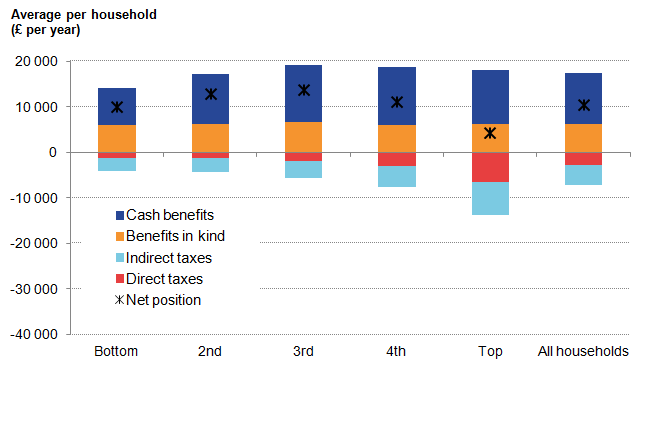
Figure 12: Summary of the effects of taxes and benefits by quintile groups, non-retired households, financial year ending 2015, UK

Source: Office for National Statistics

Download this image Figure 12: Summary of the effects of taxes and benefits by quintile groups, non-retired households, financial year ending 2015, UK

.png (14.5 kB) .xls (19.2 kB)

In 2014/15, only the bottom two-fifths of non-retired households were net beneficiaries of the taxes and benefits system (Figure 12). Across the income distribution, benefits in kind were the largest component of the benefits received. The poorest fifth of non-retired households received one of the highest values from these benefits, on average £8,700 per year in 2014/15.

97% of benefits in kind for all non-retired households were due to benefits arising from education and the National Health Service (NHS), though the relative importance of each of these varied across the income distribution. For the bottom two-fifths, education was the largest single benefit in kind, reflecting the composition of households in this part of the distribution, which had the highest number of children per household on average (Effects of taxes and benefits dataset Table 5). For the remaining three-fifths, the NHS contributed the most to the total benefits in kind on average. Again, this reflects the composition of households at this end of the income distribution. A larger percentage of households in these quintiles had a chief economic supporter⁶ aged over 64.

Notes for Longer-term trends in income inequality

1. The chief economic supporter is the person in the household who contributes most to the household income.
2. Throughout this release, 2014/15 refers to the financial year ending 2015 and similarly for other years in this format.

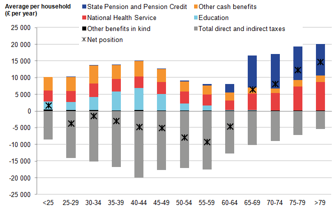
The effects of taxes and benefits are felt differently by households in different age groups (Figure 13). On average, in 2014/15 households with a household head aged between 25 and 64 paid more in taxes (direct and indirect) than they received in benefits (including in-kind benefits), whilst the reverse was true for those aged 65 and over. Those with a household head in their early 40s on average paid the most in taxes (£19,800) but also received the highest benefits of those below State Pension age (£15,000), due mainly to the benefit received from state-provided education (£6,600).

For households with heads aged 65 and over, the State Pension/pension credit was the largest component of the benefits received, followed by the benefit derived from the National Health Service, which becomes increasingly important as age increases.

Those households with heads under the age of 25 were the other age group who, on average, received more in benefits than they paid in taxes.

Figure 13: The effects of taxes and benefits by age of the head of the household, financial year ending 2015, UK

Source: Office for National Statistics

Download this image Figure 13: The effects of taxes and benefits by age of the head of the household, financial year ending 2015, UK

.png (24.0 kB) .xls (10.8 kB)

The impact of taxes and benefits on redistributing income for households in different age groups can be seen when comparing income at the different stages of redistribution for these households (Figures 14a for 2014/15 and 14b for 10 years earlier as a comparison). This shows that there is much less variation across different age groups in either average disposable or final income, than there is in original income.

In 2014/15, for households with heads aged 25 to 64, on average, their original income (before any taxes and benefits) is higher than their disposable income. However, this picture changes for those with heads over the age of 65, where average disposable income exceeds original income.

For most age groups, average final income is relatively close to disposable income. One exception is among those households with heads between the ages of 50 and 64, where average final income is lower, reflecting in part the lower in-kind education benefits received compared with younger households, due to a smaller proportion of households with school age children. The other main exception is for those households with heads aged 75 or above, for whom NHS services become increasingly valuable, increasing the average value of final income.

The pattern observed in the 2014/15 data is very similar to that seen in 2004/05. The main difference is that, in 2004/05, average original and disposable incomes were highest for households with heads aged 50 to 54, with incomes starting to fall for older age groups. By contrast, in 2014/15, incomes remained at a similar level for households with heads aged 55 to 59. This may be due in part to differences in the proportion of households with heads aged 55 to 59 who are retired or otherwise not economically active.

Notes for The effects of taxes and benefits across the life cycle

1. Throughout this release, 2014/15 refers to the financial year ending 2015 and similarly for other years in this format.

In the financial year 2014/15, outcomes in the labour market are likely to have directly affected household incomes. In the 3 months to March 2015, both the number of people in employment (31.1 million) and the headline employment rate (73.5%) were at their highest levels since records began. The unemployment rate, which fell by 1.0 percentage point in the year to Quarter 1 (Jan to Mar) 2014, fell by a further 1.3 percentage points in the year to Quarter 1 (Jan to Mar) 2015 to reach 5.5%, while the experimental Claimant Count rate, which fell 1.3 percentage points in the year to March 2014, fell further in the year to March 2015, by 1.0 percentage point to reach 2.3%. The proportion of those aged over 16 who were inactive was broadly unchanged over this period. These series together point towards greater job security and therefore household confidence during this period. This evidence also suggests developing labour market conditions boosted household incomes over this period, by increasing the number of people in work.

Alongside this growth in employment, wages also began to show signs of recovery during this period. In the 3 months ending March 2015, annual wage growth was 2.3%, which was 1 percentage point higher than over the same period of 2014. Wage growth was stronger in finance and business services (3.2%) and in wholesale, retailing, hotels and restaurants (3.2%), and weaker in manufacturing (0.7%) over this period. Private sector pay growth, at 2.8%, was also stronger than in the public sector (excluding financial services), where pay grew by 1.3%. All else being equal, this evidence of tightening in the labour market coupled with wage growth implies that the amount paid in taxes per person increased in the financial year 2014/15 and the amount claimed in benefits decreased.

Stronger nominal wages have also raised the growth rate of real earnings as prices changed little on average between 2013/14 and 2014/15 (Figure 15). Inflation, as measured by the Consumer Prices Index (CPI), was 0.0% in the year to March 2015, the lowest rate ever recorded and 1.6 percentage points lower than the previous year. Over the period between Quarter 2 (Apr to June) 2014 and Quarter 1 (Jan to Mar) 2015, the household final consumption expenditure measure of prices (the HHFCE implied deflator), which indicates the price changes that households faced when purchasing a broader range of products, grew by 0.2%, a fall of 1.1 percentage points compared with the same period in 2013/14.

The low inflation experienced during this period, combined with the recovery in nominal wages, led to a resurgence in real wages and therefore purchasing power during the 2014/15 financial year. Annual regular pay growth in real terms (3 month average) was negative between July 2008 and September 2014, became positive in October 2014 and increased to 2.2% in March 2015, its highest rate since November 2007.

In broader terms, the UK economy continued to grow in the financial year 2014/15, continuing the recovery which started in Quarter 3 (July to Sept) 2009. By the end of this period there had been 9 quarters of consecutive increase in GDP. However, the growth rate of GDP eased from 2.2% in the financial year 2013/14, to 1.7% in 2014/15. By Quarter 1 (Jan to Mar) 2015, UK GDP was 5.0% above its pre-downturn peak in Quarter 1 (Jan to Mar) 2008. GDP per head – which has recovered more slowly – was 0.3% below its pre-downturn peak by Quarter 1 (Jan to Mar) 2015.

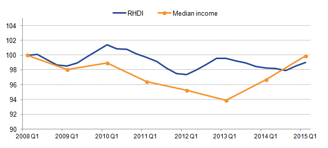
Figure 16: Real median equivalised household disposable income and real household disposable index (RHDI) per head, excluding non-profit institutions serving households (NPISH), Quarter 1 (Jan to Mar) 2008 to Quarter 1 (Jan to Mar) 2015, UK, Index Quarter 1 2008=100

Source: Office for National Statistics

Download this image Figure 16: Real median equivalised household disposable income and real household disposable index (RHDI) per head, excluding non-profit institutions serving households (NPISH), Quarter 1 (Jan to Mar) 2008 to Quarter 1 (Jan to Mar) 2015, UK, Index Quarter 1 2008=100

.png (11.0 kB) .xls (27.1 kB)

In early 2015, both median household disposable income and RHDI per head were at similar levels to those seen in early 2008. However, the paths of these measures have been notably different since early 2008. Median household disposable income fell 6.1% between the financial year 2007/08 and 2012/13 before recovering between 2012/13 and 2014/15. Figure 16 shows that changes in RHDI per head have been less pronounced; as RHDI has remained within 3% of its Quarter 1 (Jan to Mar) 2008 level during this period.

The deviation in the paths of the 2 measures in 2009 is likely to be due to the impact of lower interest rates during this period. While median household income includes gross interest receipts – which fell markedly during the downturn – RHDI includes a net measure of interest received which offset the fall in interest receipts with the reduction in interest paid by households. As a consequence, the net income measure in RHDI was more resilient over this period. Since 2013, however, median household income has grown more strongly than RHDI per head – likely reflecting the rising employment rate over this period, which in turn has increased median earnings per household. While RHDI has also been affected by the higher employment rate, it has a much larger impact on a median income measure, than on a measure of aggregate household income such as RHDI.

Notes for Economic context

1. Throughout this release, 2014/15 refers to the financial year ending 2015 and similarly for other years in this format.