1. Abstract
This article presents the results of 2 statistical models which explore the relationship between mean hourly earnings excluding overtime and a range of independent variables. The findings are based on Annual Survey of Hours and Earnings – 2016 provisional results data. There is a particular focus on earnings differences between the public and private sectors. One model includes organisation size as an independent variable and one excludes this factor.
Back to table of contents2. Main points
Public and private sector pay differences
Looking across the employees in the Annual Survey of Hours and Earnings (ASHE) dataset the mean pay in the public sector is estimated to be 1.0% less than in the private sector in 2016. This uses the model which excludes organisation size and controls for a range of independent variables including region, occupation, age, gender and job tenure. This continues a downward trend seen since 2012 and is the first year in the series that the differential is in favour of the private sector since 2003.
In the model which includes organisation size, the mean pay in the public sector is estimated to be 5.5% less than in the private sector in 2016.
Looking at the top and bottom of the pay scale we see divergence between public and private pay. Public sector pay is estimated to be 10.8% above private sector pay at the bottom of the earnings distribution (5th decile), but 13.2% below private sector pay at the higher end of the earnings distribution (95th decile), when using an identically specified quantile regression model excluding organisation size.
The gap at the top of the earnings distribution between public and private sector employees has been increasing over time, but narrowing at the bottom of the earnings distribution.
In the quantile regression model which includes organisation size, the same trend exists across the earnings distribution but shows lower earnings in the public sector at each quantile.
Other factors affecting pay at the mean of the earnings distribution
In the model which excludes organisation size, part-time workers in 2016 are estimated to earn 8.8% less than full-time workers and temporary workers earned 0.7% less than permanent workers.
The corresponding figures are 6.5% less for part-time workers and 2% less for temporary workers respectively in 2016 in the model which includes organisation size.
The model which excludes organisation size estimates the North East and North West, for example, to have average pay around 6 to 7% lower than London in 2016. The equivalent figures for these regions using the model including organisation size are 5 to 6% lower than London.
Back to table of contents3. Introduction
Headline measures of median weekly earnings for full-time employees in the UK are published in Annual Survey of Hours and Earnings - 2016 Provisional Results. These data are useful for comparing groups of employees but do not take into account the different composition and characteristics of these employees. For example, comparing median earnings between employees in the public and private sectors, or between men and women does not take into account the additional factors that are common to these groups, such as the public sector having generally older workers than the private sector, or more women working in certain occupations compared with men.
This article updates the previous regression results published last year and addresses this issue. It presents the results of a regression model, developed in 2011 by the Office for National Statistics (ONS) and HM Treasury, which statistically controls for a range of factors related to earnings that are available in the ASHE dataset. This enables the influence of separate factors on hourly earnings to be identified, such as working in the public or private sectors while keeping other predictive factors constant.
There are 2 variants of the regression model presented in this article – one excluding and one including organisation size. The analysis from this model gives estimates of mean hourly pay controlling for a range of independent variables available in the ASHE dataset. In addition, identically specified quantile regression models – with and without organisation size – are used to give estimates of hourly pay at different points in the earnings distribution, including the median.
There are a number of important points to note about this analysis and the approach used in the regression model (further information on the regression methodology is given in the statistical notes to this article):
the ASHE dataset only covers the earnings of paid employees in the UK and does not include data on self-employed earnings (who are often some of the highest paid workers, as well as some of the lowest paid workers)
the dependent variable of the statistical model is hourly earnings excluding overtime pay; overtime paid at a higher rate would increase an employee’s hourly pay whereas working unpaid overtime would effectively reduce hourly pay
an adjustment is made to hourly earnings in the ASHE dataset using the Average Weekly Earnings series (published monthly based on the Monthly Wages and Salaries Survey) to better account for the timing of bonus payments throughout the year; estimates in this article are not therefore directly comparable with those published in ASHE Provisional Results 2016 which do not make this adjustment for the timing of bonus payments
pension contributions or other forms of remuneration such as company car or health insurance by employers are not yet available in the 2016 ASHE dataset and the regression model has not been designed to take them into account
for April 2016, as for April 2015, the private sector element excludes employees in the non-profit institutions serving households (NPISH); in the UK the NPISH sector includes organisations such as charities, trade unions and most universities; in some other surveys this group is included in the analysis of private sector organisations and employees – this treatment, however, is consistent with previous analysis of ASHE data
for consistency over time, employees of those banks classified to the public sector in 2008 have been treated as if they were in the private sector throughout
The estimates in this article are dependent on the specification of the statistical models and including additional or alternative independent variables would give different results. The model currently explains over half of the variation in earnings. Data important to earnings such as education level is also not available in the ASHE dataset and limits some of the interpretation of results.
This article is split into 2 sections:
Section A describes the factors which are used in the earnings regression model using the provisional ASHE dataset for April 2016
Section B discusses the main results from the 2 linear and 2 quantile regression models – with and without organisation size – with a particular focus on the differences between public and private sector earnings
4. Section A: Factors affecting earnings
This section will consider a number of factors that are taken into account analysing earnings. Simple averages are considered to gain an initial insight into pay differences amongst individuals with different characteristics (such as age and gender) and job-related characteristics (such as public or private sector, occupational group, region of employment, job tenure, job status and size of employer).
Individual characteristics
Age and sector
Age is an important factor affecting earnings, as this tends to be a proxy for experience and the build-up of skills over time. Figure 1, although not accounting for the different jobs within each sector, shows that the age profile of workers varies significantly by whether they are employed in the public or private sector.
The distribution of jobs held within the private sector is more skewed towards younger age groups, while the distribution of jobs held within the public sector is more skewed towards older age groups. The fall in the share of employees for both sectors around the 30s age group is a reflection of population demographics.
Mean hourly pay for all employees, regardless of sector, rises sharply at younger ages as job-related skills and experience is rewarded. Peaking in both sectors at around age 42, the average private sector wage level remains slightly higher than the public sector average between the ages of 38 and 53 years. Average private sector pay then declines faster after this age compared with the public sector.
Figure 1: Mean hourly earnings and share of all employees by age and sector, April 2016
UK

Source: Annual Survey of Hours and Earnings (ASHE) - Office for National Statistics
Notes:
- Data for 2016 is provisional.
Download this image Figure 1: Mean hourly earnings and share of all employees by age and sector, April 2016
.png (22.1 kB) .xls (21.5 kB)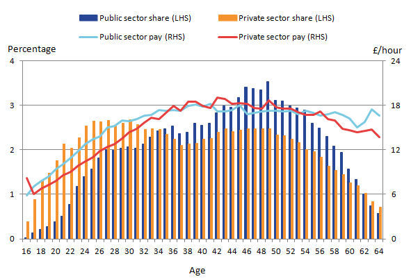
Age, gender and sector
A similar analysis of the distribution of jobs held by men and women at each age is given in Figure 2. This shows a relatively equal age distribution for men and women from around 20 to 28 years old. However, the female employment share drops by around a third between the ages of around 28 years to around 40 years likely to coincide with women taking time out to raise a family.
The female employment share then starts to increase from age 40 onwards until age 52 without seeing the same increase in average hourly earnings. In fact earnings are seen to slightly decrease with age for women after their mid 30s whereas for men any earnings decline is not seen until the early 50s. The employment share of men and women at older ages decreases at similar rates.
Figure 2: Mean hourly earnings and share of all employees by age and gender, April 2016
UK

Source: Annual Survey of Hours and Earnings (ASHE) - Office for National Statistics
Notes:
- Data for 2016 is provisional.
Download this image Figure 2: Mean hourly earnings and share of all employees by age and gender, April 2016
.png (25.9 kB) .xls (22.5 kB)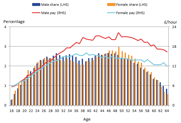
As already highlighted, there are differences in earnings between the sectors related to the age of the employees. There are also differences in earnings between the sectors when split by gender (Table 1).
Table 1: Average earnings per hour by gender and sector, April 2016, UK
| Male earnings (£/hour) | Female earnings (£/hour) | % of females in sector | |
| Public sector | 19.09 | 15.33 | 67.6 |
| Private sector | 17.19 | 12.34 | 42.5 |
| Source: Annual Survey of Hours and Earnings (ASHE) - Office for National Statistics | |||
| Note: | |||
| 1. Data for 2016 is provisional | |||
| 2. All employees including those on junior rates and those affected by absence | |||
Download this table Table 1: Average earnings per hour by gender and sector, April 2016, UK
.xls (27.1 kB)Women make up over two-thirds of public sector employees compared with 42.5% of employees in the private sector, but on average are paid less than men in the public sector. Similarly, women are paid less than men on average in the private sector. To better understand these differences in earnings it will be important to control for occupation, job tenure and other factors as we do in section B.
Job-related characteristics
Occupation, skill group and sector
Earnings are likely to increase as the skill level of the job increases. Thus differences in pay by sector may be partly explained by compositional differences in the share of employees at each skill level. In this instance, skill is defined solely by occupation and is grouped into 4 broad skill levels using the Standard Occupational Classification (SOC 2010). Professional or upper skill group jobs include occupations such as scientists, IT engineers, health and educational professionals, while elementary occupations or lower skill group occupations include farm workers, window cleaners, waiters, waitresses and processing operatives. The background notes provide more detail of occupations in each skill group.
Figure 3: Occupational skill share of employee jobs by sector, April 2016
UK
Source: Annual Survey of Hours and Earnings (ASHE) - Office for National Statistics
Notes:
- Data for 2016 is provisional.
Download this chart Figure 3: Occupational skill share of employee jobs by sector, April 2016
Image .csv .xlsFigure 3 shows a compositional effect in that a larger proportion of public sector employees are in the professional and upper middle skilled group (75%) compared with the private sector (48%). The remaining 52% of private sector employees are in the lower middle and lower skills group.
Region and occupation group
Figure 4 shows the mean hourly pay for employees (aged 16 to 64 years) and mean hourly pay for employees in professional occupations and employees in elementary occupations.
There are differences in average hourly pay across the regions, particularly for professional occupations in the South East and London. Professionals in London earn on average nearly £12 per hour more (57%) than their Northern Ireland counterparts and over £1 per hour (15%) more in elementary occupations. For these regions, the higher average hourly pay for all workers is due to the pay of professional occupation workers rather than elementary occupation workers and points to relatively large levels of inequality of earnings within London – professional occupations earn on average, around 3.7 times more per hour than elementary occupations in London. This compares with a ratio of average earnings of professional occupations to elementary occupations of 2.6 to 2.9 in other regions and countries of the UK. The varying nature of work and other factors may be the cause for differences in average hourly earnings between London and other regions although other factors such as living costs may also contribute to these variations.
Figure 4: Mean hourly earnings by region for all employees, elementary and professional occupations, and National Living Wage, April 2016
UK
Source: Annual Survey of Hours and Earnings (ASHE) - Office for National Statistics
Notes:
- Data for 2016 is provisional.
Download this chart Figure 4: Mean hourly earnings by region for all employees, elementary and professional occupations, and National Living Wage, April 2016
Image .csv .xlsWorking patterns and sector
The additional factors of whether a job is full-time or part-time and whether it is permanent or temporary also has an influence on earnings. Table 2 shows that mean hourly earnings in April 2016 of full-time employees was on average £3.30 higher than for part-time employees in the public sector, but this difference is higher at around £7.20 in the private sector.
On average in 2016, employees in permanent jobs earn more per hour than those in temporary or casual jobs. Within the public sector this is £1.20 more on average whereas in the private sector this was around £5.30 more.
There is a larger share of part-time working in the public sector compared with the private sector (30% of employee jobs compared with 25% in the private sector) and use of temporary jobs (10% of public sector employee jobs compared with 7% of private sector jobs). These shares are unchanged from 2015.
Table 2: Mean hourly earnings by job characteristic, and share of jobs by sector, April 2016, UK
| Earnings (£/ hour) Public sector | Share of employee jobs in public sector (%) | Earnings (£/hour) private sector | Share of employee jobs in private sector (%) | |
| Full-time | 17.56 | 70 | 16.97 | 75 |
| Part-time | 14.26 | 30 | 9.77 | 25 |
| Permanent | 16.68 | 90 | 15.51 | 93 |
| Temporary | 15.48 | 10 | 10.19 | 7 |
| Source: Annual Survey of Hours and Earnings (ASHE) - Office for National Statistics | ||||
| Note: | ||||
| 1. Data for 2016 is provisional | ||||
Download this table Table 2: Mean hourly earnings by job characteristic, and share of jobs by sector, April 2016, UK
.xls (27.1 kB)Longer job tenure, as defined as length of time with current employee, is associated on average with higher pay in both the public and private sectors. At shorter tenures of roughly 5 years or less however, public sector workers have higher average pay than private sector workers. Private sector workers have higher average pay at tenures longer than 5 years. Individuals that work in the public sector are more likely to have worked for long tenures than those in the private sector, with over one quarter of public sector employees having worked for their employer for between 10 and 20 years. Within the private sector the modal tenure length is between 2 and 5 years (representing just over one-fifth of private sector employees).
Size of organisation
The size of the employer organisation can influence rates of pay. Larger employers may be able to pay higher wages for similar roles than smaller ones, as larger organisations may have higher profit margins or greater efficiencies of scale.
Figure 5 shows that in April 2016, a total of 58.2% of all employee jobs were in organisations with over 500 employees (up 0.9% from 2015) with noticeable differences between the public and private sectors. The public sector tends to be concentrated in large organisations with at least 500 employees, with around 90% of public sector employees working in these large organisations. Such organisations include the NHS, fire and police services or local authorities. In contrast, there is a much more even split of employees across the organisation sizes for the private sector, with just under half working in large organisations in 2016. Around 12% of private sector employees worked in organisations of 10 employees or fewer, whereas for the public sector this was just 0.2%. People who work in small and large organisations differ across the economy.
Figure 5: Percentage of employee jobs by size of organisation and by sector, April 2016
UK
Source: Annual Survey of Hours and Earnings (ASHE) - Office for National Statistics
Notes:
- Data for 2016 is provisional.
Download this chart Figure 5: Percentage of employee jobs by size of organisation and by sector, April 2016
Image .csv .xlsEarnings distribution by sector
Finally, Figure 6 shows that the earnings of the public sector are generally higher for all employees across the earnings distribution, apart from the top 10% of earners. In April 2016 specifically, mean hourly public sector pay exceeded private sector pay by between £0 to £5 per hour until the 88th percentile of the pay distribution. At this point mean public sector pay was £25.23 per hour, and mean private sector pay was £25.58. In April 2016, private sector employees at the 99th percentile of earnings were paid around £20 per hour more than employees at the 99th percentile of hourly earnings in the public sector.
These data show the value of presenting quantile regression results which identify pay differences at the median and other points in the earnings distribution.
Figure 6: Distribution of hourly earnings in the public and private sector, April 2016
UK
Source: Annual Survey of Hours and Earnings (ASHE) - Office for National Statistics
Notes:
- Data for 2016 is provisional.
Download this chart Figure 6: Distribution of hourly earnings in the public and private sector, April 2016
Image .csv .xlsNotes for Section A: Factors affecting earnings
Part time is defined as employees working 30 paid hours per week or less.
This includes NPISH sector employees and those unclassified by sector.
5. Section B: Regression analysis modelling pay differences
Specification
Comparison of average pay differentials made in section A can create a partial picture, as employees have multiple personal and job characteristics that can impact on their pay. Regression modelling can be used to account for some of these differences by including controls for them. This regression analysis estimates the pay difference between types of individuals when controlling for the following factors.
Data source and variable filters applied
The primary source of data is the Annual Survey of Hours and Earnings (ASHE) using hourly earnings (excluding overtime) for all employees whose pay in the April period was not affected by absence and were paid adult rates. This data has been adjusted to account for bonus payments paid outside of the period covered by ASHE using data from the Average Weekly Earnings (AWE) series.
Regression model specification
Dependent variable:
- log of bonus-adjusted hourly earnings excluding overtime (see statistical note 1 and 4)
Independent variables:
sex – there is a difference in the distribution of men and women in the public and private sector
age and age squared – the relationship between earnings and age is non-linear (see statistical note 2)
occupation classification, these are narrower than in section A (see background notes)
region (regions of job location) – the proportion of jobs in each sector varies by region
sector (public or private)
full- or part-time status – the difference in pay and the difference in proportion varies between sectors
permanent or temporary status – the distribution of these is different between sectors and the difference in pay is different between sectors
job tenure – less or equal to 6 months, 6 to 12 months, 1 year to 2 years, 2 to 5 years, 5 to 10 years, 10 to 20 years and over 20 years – job tenure is a proxy for organisation-specific experience
Interaction terms: (see statistical note 3)
sex*age and sex*age squared – the potential work experience proxied by age for males and females is different, that is, women experience more career interruptions than males
occupation*age and occupation*age squared – the return to work experience may be different for different occupations
occupation*region – industry and labour market structures that impact on wages differ between regions
In the model controlling for organisation size1 we also include as explanatory variables:
organisation size, categorised into 6 bands by number of workers: less than or equal to 10, 11 to 25, 26 to 50, 51 to 250, 251 to 500, 501 and over
organisation size*occupation – the effect of organisation size on pay may differ for different occupation classifications
The Analysis of factors affecting earnings using the Annual Survey of Hours and Earnings linear regression dataset gives the coefficients generated by the linear regression model and provides metadata for the variable names and model specifications. The statistical notes in this section explain how to interpret these results.
Differences in private and public sector pay
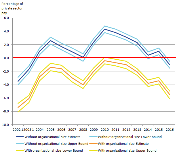
Figure 7: Average difference in mean hourly pay (excluding overtime) between public and private sector workers expressed as a percentage of private pay, April 2002 to April 2016
UK
Source: Annual Survey of Hours and Earnings (ASHE) - Office for National Statistics
Notes:
- No data is available for Northern Ireland for 2002 to 2003, estimates for these years refer to Great Britain.
- Data for 2016 is provisional.
Download this image Figure 7: Average difference in mean hourly pay (excluding overtime) between public and private sector workers expressed as a percentage of private pay, April 2002 to April 2016
.png (50.6 kB) .xls (31.2 kB)
Comparing sectors and controlling for the variables set out earlier in this section, Figure 7 shows the average difference and 95% confidence intervals in hourly pay between public and private sector workers expressed as a percentage of private sector pay between April 2002 and 2016 (see statistical note 5 for its calculation method). A positive number indicates a pay gap in favour of the public sector and a negative number indicates a pay gap in favour of the private sector.
The model results, controlling for the factors listed in section A, provide the opposite result to that described in section A (where it was found hourly earnings in the public sector were greater than in the private sector). The model results excluding organisation size show 2016 is the first year since 2003 in which the public sector earns less than the private sector; by 1%. There has been a steady reduction in the pay premium for the public sector since 2010, the premium moving in favour of the private sector in 2016.
The model controlling for organisation size shows that public sector employees earn on average 5.5% less than employees in the private sector in 2016. This gap has widened from 2015 when it was 3.4%. In this model, the pay differential in favour of the private sector has been increasing since 2010 (increasingly negative public sector coefficients).
It is therefore implied in both cases – with and without organisation size included in the regression model – that growth in mean hourly earnings for employees in the private sector has grown faster (all other factors being equal) than in the public sector between 2015 and 2016. This may be a reflection of restrictions on public sector pay increases for 2015 to 2016 announced in Budget 2013 and generally faster growth in pay in the private sector during this time. For example, between April 2015 and April 2016, pay growth was 3.3% in the private sector compared with 1.8% for the public sector (Average Weekly Earnings, EARN02 dataset).
Quantile regression results
The Analysis of factors affecting earnings using the Annual Survey of Hours and Earnings quantile regression dataset gives the coefficients generated by the quantile regression models and provides metadata for the variable names and model specifications. The statistical notes in this section explain how to interpret these results.
The linear regression model considers the difference in the mean pay of public and private sector workers. This does not take account of the fact that the distribution of pay tends to be narrower in the public sector than the private sector and so does not give a complete picture.
It is possible to use quantile regression methods to estimate the difference in the median pay of public and private sector workers as well as the difference at each percentile, for example, the 5th or 10th percentile. This is useful as it indicates if the pay gap is different at different points of the pay distribution, effects which cannot be captured by mean regressions.
It should be noted that estimates across different quantiles of the income distribution compare the average hourly pay for a certain distribution of the public sector workforce to the average pay for a certain distribution of the private sector workforce. For example, if we observe a positive public sector premium at the lower end of the distribution, this does not necessarily imply that if an individual in this part of the income distribution working in the public sector was to move to the private sector, they would earn a lower hourly pay. Instead it implies that individuals in the lower end of the public sector income distribution – conditional on observed characteristics – earn an hourly premium compared with the individuals in the lower end of the private sector income distribution.
The pay gap between private and public sector workers has been estimated for the 2nd, 5th and 10th percentiles, the median and the 90th, 95th and 98th percentile for 2012 to 2016, using the quantile regression model both excluding and including organisation size.
Table 3 shows the difference in hourly pay between public and private sector workers expressed as a percentage of private pay by percentile for April 2012 to 2016, where a positive number indicates the pay gap is in favour of the public sector.
Table 3: Quantile and mean regression results for differences in public sector pay as a percentage of private sector pay, 2012 to 2016
| Percentile | ||||||||
| Year | 2nd | 5th | 10th | 50th | 90th | 95th | 98th | Mean |
| Without organizational size | ||||||||
| 2012 | 12.9 | 13.1 | 12.4 | 6.3 | -3.3 | -5.9 | -9.9 | 3.1 |
| 2013 | 12.3 | 12.6 | 11.9 | 4.7 | -3.2 | -6.4 | -10.6 | 2.3 |
| 2014 | 10.7 | 11.6 | 11.0 | 2.6 | -4.8 | -7.4 | -10.4 | 0.4 |
| 2015 | 13.1 | 12.9 | 11.4 | 1.1 | -9.9 | -11.2 | -13.9 | 1 |
| 2016 | 10.9 | 10.8 | 10.0 | 0.4 | -10.9 | -13.2 | -17.2 | -1 |
| With organizational size | ||||||||
| 2012 | 9.2 | 9.5 | 9.0 | 2.5 | -7.2 | -9.9 | -13.9 | -1 |
| 2013 | 8.0 | 8.4 | 8.3 | 1.1 | -7.4 | -10.9 | -15.3 | -2.1 |
| 2014 | 6.6 | 7.5 | 7.2 | -0.7 | -9.2 | -11.7 | -14.2 | -3.8 |
| 2015 | 8.1 | 7.7 | 7.1 | -3.4 | -14.1 | -16.0 | -19.0 | -3.4 |
| 2016 | 6.8 | 6.8 | 5.8 | -4.3 | -15.4 | -17.7 | -21.5 | -5.5 |
| Source: Annual Survey of Hours and Earnings (ASHE) - Office for National Statistics | ||||||||
| Note: | ||||||||
| 1. Data for 2016 is provisional | ||||||||
Download this table Table 3: Quantile and mean regression results for differences in public sector pay as a percentage of private sector pay, 2012 to 2016
.xls (28.2 kB)In 2016, both the model controlling for and not controlling for organisation size indicate that the pay gap is wider at the top end of the distribution than the bottom. There have also been changes at the 50th percentile (median) where the size of the gap has been decreasing.
For instance at the 5th percentile, public sector workers earned 6.8% (10.8% in the model without organisation size) more on average than private sector workers in 2016. At the other end of the pay distribution, at the 95th percentile, public sector workers earned 17.7% (13.2% in the model without organisation size) less on average than private sector workers in 2016. From 2012, the pay gap on average has been narrowing at the lower end of the distribution and increasing at the higher end.
The pay gap in favour of the public sector at the bottom of the distribution may be due to the private sector having more jobs paid close to the National Minimum Wage than the public sector. In comparison, the pay gap in favour of the private sector at the top of the distribution can be explained by the fact that the public sector, in general, does not have the very high wages at the top of the wage distribution as seen in the private sector.
Analysis of other factors
In addition to sector, the linear regression model in 2016 found almost all other variables within the model were statistically significant at the 1% level.
Working pattern
One of the largest impacts on earnings, with all other factors being equal, comes from an employee’s job tenure – how long an employee has been in their current job. Figure 8 compares the pay differential of the job tenure groups with those who have been in their job for 6 months or less and suggests that the longer a person is in a job, the more they earn, allowing for all other individual and job-related factors such as gender, occupation and region.
At the same time the model suggests this relationship holds with each subsequent group earning more than the previous group, up to those in the same job for 20 years or more earning 22.3% more than those newly started in a job.
Figure 8: Average difference in mean hourly pay (excluding overtime) by job tenure group, aged 16 to 64, 2016
UK
Source: Annual Survey of Hours and Earnings (ASHE) - Office for National Statistics
Notes:
- Data for 2016 is provisional.
- This percentage is the difference in pay compared with the reference group. .
- The reference group is those that have been employed for less than 6 months.
- Results are significant at a 1% level.
Download this chart Figure 8: Average difference in mean hourly pay (excluding overtime) by job tenure group, aged 16 to 64, 2016
Image .csv .xlsControlling for all other factors, including public and private sectors, in the model which excludes organisation size, part-time workers in 2016 earned 8.8% less than full-time workers when controlling for other factors and temporary workers earned 0.7% less than permanent workers. In the model which includes organisation size in 2016, the figures are 6.5% less for part-time workers and 2% less for temporary workers respectively.
Organisation size
The model including organisation size observes the effect of how large a firm someone is employed in, on their earnings. In 2016, relative to employees in organisations with more than 500 employees, those employed in all breakdowns of smaller firms earn relatively less on average. Specifically, employees in organisations with between 11 and 55 employees earn between 8 to 9% less than organisations with more than 500 employees. For larger organisations (with between 50 and 499 employees) the earnings penalty is 4 to 6% on average. The pay differentials are not as regressive as other variables observed, with the impact being much more uniform amongst firms of differing size.
Regional variation
Table 4: Average difference in mean hourly pay (excluding overtime) between London employees and other regions of England and the devolved administrations of the UK
| Percentage difference in average hourly pay to London | ||
| Region | Excluding organisation size | Including organisation size |
| North East | -7.04 | -5.91 |
| North West | -5.68 | -4.88 |
| Yorkshire and The Humber | -6.18 | -5.20 |
| East Midlands | -5.09 | -4.38 |
| West Midlands | -5.40 | -4.68 |
| South West | -4.34 | -3.58 |
| East | -5.40 | -4.52 |
| South East | ||
| Wales | -7.22 | -6.07 |
| Scotland | -2.37 | |
| Northern Ireland | -10.32 | -8.50 |
| Source: Annual Survey of Hours and Earnings (ASHE) - Office for National Statistics | ||
| 1. Data for 2016 are provisional | ||
| 2. All results are significant at the 1% level other than for the South eaast which shows no statistical difference | ||
Download this table Table 4: Average difference in mean hourly pay (excluding overtime) between London employees and other regions of England and the devolved administrations of the UK
.xls (28.2 kB)Table 4 shows the difference in pay between London and the rest of the UK for the linear regression model including andexcluding organisation size. The model which excludes organisation size estimates the North East and North West, for example, have average pay around 6 to 7% lower than London in 2016 when controlling for other factors. The equivalent figures for these regions using the model including organisation size are 5 to 6% lower than London.
Conclusion
The estimates presented in this article are by no means a definitive measure of earnings. In fact the model explains 55% of the difference in earnings between people. A different model containing additional or alternative independent variables may explain more of the variation. However, it is not possible to include all factors that affect pay, such as employee ability or motivation, as information on these factors is not available. In addition these are estimates based on a sample such that different samples would give different results.
Notes for Section B: Modelling pay differentials in the public and private sector:
- The logic for a creating model that includes organisation size and another that does not is as follows. Firstly, if the view is held that public sector employees should earn the same as private sector employees irrespective of organisation size, then it would be useful to see the results without organisation size included. From a statistical point of view, as over 90% of those working in the public sector are also in large organisations thus the inclusion of organisation size can lead to issues of collinearity and have an impact on the precision of the estimate of the public and private sector pay differential. The model with organisation size, however, still remains statistically valid.
6. Statistical notes
The dependent variable is expressed in log form. If the distribution of a variable has a positive skew, taking a natural logarithm of the variable sometimes helps fitting the variable into a model. Also, when a change in the dependent variable is related with percentage change in an independent variable, or vice versa, the relationship is better modelled by taking the natural log of either or both of the variables.
When accounting for the age of employees in the regression model, we have incorporated a variable for both age and age squared; this is due to the Taylor series approximations. Taylor series approximations tell us that for many smooth functions, they can be approximated by a polynomial, so including terms like Χ2 or Χ3 let us estimate the coefficients for the approximation for a known or unknown non-linear function of Χ, or in this case age.
As well as the suite of independent variables observed in the model, a number of interaction terms are included. These are added to account for the assumption that some characteristics interact with one another.
The presence of a significant interaction indicates that the effect of the first independent variable (α1) on the dependent variable (Ω) is different at different values of a second independent variable (α2). It is tested by adding a term to the model in which the 2 independent variables are multiplied.
Ω = A + β1*α1 + β2*α2 + β3*α1*α2
Adding an interaction term to a model drastically changes the interpretation of all of the coefficients. If there were no interaction term, β1 would be interpreted as the unique effect on the Ω(in this case pay). But the interaction means that the effect of α1 Ωon is different for different values of α2. So the unique effect of 1 is not limited to β1, but also depends on the values of β3 and α2.
The unique effect of 1 is represented by everything that is multiplied by α1 in the model:
β1 + β3* α2. β1 is now interpreted as the unique effect of α1 on Ω only when α2= 0.
When interpreting the outputs of the model, care needs to be taken with the coefficients of variables. While the independent variables are in their original state, the dependent variable is in its log-transformed state, therefore, the coefficient (β) for the independent variables do not simply reflect the percentage change but (100*β)% for a one unit increase in the independent variable, with all other variable in the model held constant.
Taking into consideration the statistical notes, the calculations conducted to estimate the pay gap between the public and private sector follow algebraically
In the final model, public or private sector is coded as:
The base category is the private sector and there is a dummy variable that codes for public sector called “_l_banks_rec_1” in the regression output.
The variable “_l_banks_rec_2” measures the unclassified pay premium relative to the private sector. This sometimes gets dropped in the regression estimation. This is important for estimation but not the focus of the analysis.
Taking model 6 and deriving the formula for the public sector pay premium. Assume other characteristics the same in Δ:
Hence
7. Background notes
Survey details
The Annual Survey of Hours and Earnings (ASHE) is based on a 1% sample of employee jobs taken from HM Revenue and Customs Pay-as-you-earn (PAYE) records. Information on earnings and hours is obtained from employers and treated confidentially. ASHE does not cover the self-employed nor does it cover employees not paid during the reference period.
Quality and Methodology Information
The Annual Survey of Hours and Earnings Quality and Methodology Information document contains important information on:
the strengths and limitations of the data
the quality of the output: including the accuracy of the data and how it compares with related data
uses and users
how the output was created
Classification of SOC 2010
The Standard Occupational Classification 2010 (SOC2010) separates the labour market into 9 major groups, based on criteria such as the qualifications, skills and experience associated with each job.
These 9 major groups can be combined further into 4 skill groups (levels 1 through 4, where level 1 indicates relatively low skill requirements and level 4 indicates relatively high skill requirements). Table 4 describes some of the important features of each skill group:
Table 5: SOC 2010 classification of skill groups and share of employees by skill group, April 2016
| Skill group | Proportion of men, ASHE 2016 | Proportion of women, ASHE 2016 | Typical occupations | |
| 1 (low) | 12 | 11 | Labourers (e.g. agriculture, construction), cleaners and basic admin workers | |
| 2 (lower-mid) | 26 | 46 | Secretaries, carers, hairdressers, cashiers, machine operatives, transport drivers | |
| 3 (upper-mid) | 31 | 16 | Skilled trade workers, associate professionals and technical occupations | |
| 4 (upper) | 31 | 27 | Professionals (e.g. teachers, doctors, scientists, engineers, managers, directors) | |
| Source: Annual Survey of Hours and Earnings (ASHE) - Office for National Statistics | ||||
| Note: | ||||
| 1. Data for 2016 is provisional | ||||
Download this table Table 5: SOC 2010 classification of skill groups and share of employees by skill group, April 2016
.xls (28.2 kB)In March 2012, the 2011 ASHE estimates were published on a Standard Occupational Classification (SOC) 2010 basis (they had previously been published on a SOC 2000 basis). Since the SOC forms part of the methodology by which ASHE data are weighted to produce estimates for the UK, this release marked the start of a new time series and therefore care should be taken when making comparisons with earlier years.
Similarly, methodological changes in 2004 and 2006 also resulted in discontinuities in the ASHE time series. On 28 February 2014 we published a methodological note explaining the impact of the change in Standard Occupational Classification on the estimates of public and private sector pay.
Relevance
The earnings information in ASHE relates to gross pay before tax, National Insurance or other deductions and excludes payments in kind. With the exception of annual earnings, the results are restricted to earnings relating to the survey pay period and so exclude payments of arrears from another period made during the survey period; any payments due as a result of a pay settlement but not yet paid at the time of the survey will also be excluded.
Most of the published ASHE analyses (that is, excluding annual earnings) relate to employees on adult rates whose earnings for the survey pay period were not affected by absence. They do not include the earnings of those who did not work a full week and whose earnings were reduced for other reasons, such as sickness. Also, they do not include the earnings of employees not on adult rates of pay, most of whom will be young people. More information on the earnings of young people and part-time employees is available in the main survey results. Full-time employees are defined as those who work more than 30 paid hours per week or those in teaching professions working 25 paid hours or more per week.
Sampling error
ASHE aims to provide high quality statistics on the structure of earnings for various industrial, geographical, occupational and age-related breakdowns. However, the quality of these statistics varies depending on various sources of error.
Sampling error results from differences between a target population and a sample of that population. Sampling error varies partly according to the sample size for any particular breakdown or “domain”.
Non-sampling error
ASHE statistics are also subject to non-sampling errors. For example, there are known differences between the coverage of the ASHE sample and the target population (that is, all employee jobs). Jobs that are not registered on PAYE schemes are not surveyed. These jobs are known to be different to the PAYE population in the sense that they typically have low levels of pay. Consequently, ASHE estimates of average pay are likely to be biased upwards with respect to the actual average pay of the employee population. Non-response bias may also affect ASHE estimates. This may happen if the jobs for which respondents do not provide information are different to the jobs for which respondents do provide information. For ASHE, this is likely to be a downward bias on earnings estimates since non-response is known to affect high-paying occupations more than low-paying occupations.
Further information about the quality of ASHE, including a more detailed discussion of coverage and non-response errors, is available on our archive website.
Re-weighting of the Labour Force Survey
Returned data from ASHE are weighted to UK population totals from the Labour Force Survey (LFS). The LFS itself has recently been reweighted, using revised UK and subnational population estimates consistent with the 2011 Census and updated population projections. We have found there to be negligible impact of this on the ASHE results. Further information on the LFS reweighting can be found on our LFS user guidance pages
Back to table of contents