1. Abstract
An important research goal at Office for National Statistics (ONS) is to investigate the use of textual data to gain insights about the economic activity of UK businesses. Motivated by this goal, this article outlines methods for using document vectorisation, dimensionality reduction, clustering and singular value decomposition to gain insight from text documents, and demonstrates the use of these methods on free-text data about businesses.
We demonstrate that this can produce valuable insights about the economic activity of the UK businesses and plan to use these methods in further research into business classifications using richer sources of data. In general, these methods will be useful in any context when processing large amounts of documents and when looking to discover relationships and patterns in the data.
Back to table of contents2. Introduction
This piece of work is inspired by a project the Office for National Statistics’ (ONS's) Big Data Team have been exploring with data extracted from Companies House. Medium- to large-sized businesses are required to submit a full accounts document to Companies House and within this document the businesses typically include a description of the function of the company. This is potentially useful information to help classify the business into its relevant UK Standard Industrial Classification 2007: UK SIC 2007 code, and may offer insight into emerging new topics in industry.
In particular, a recommendation of the Bean Review of Economic Statistics is that “ONS should be proactive in pressing the case for the next industrial classification system to provide a richer picture of services activity”, and using text data about businesses to classify businesses in new ways may help provide evidence for the need for this extra granularity.
The aim of the research described in this article is to explore methods for using textual data about businesses (described in section 3) to automatically generate a sentence describing the business to help inform business classification. This is challenging for a number of reasons; in particular, we are using “strings” of information rather than numerical features. The initial aim is then to convert the strings of information into some numerical features, which we call word or document vectorisation. A naive approach to do this is to embed the documents based on their word count. For example, if we have a small dictionary set of words, such as:
D = {"I", "do", "not", "like", "to", "cake", "eat", "no"},
we could represent the string “I like to eat cake” by the following row vector:
V = [1,0,0,1,1,1,1,0],
where the vector contains a ‘1’ if the string contains the word in the respective dictionary position or a ‘0' if it does not. This naive approach could work well in some situations, for instance, just discovering similarities based on the frequency of certain words, but a more sophisticated approach will also incorporate information from neighbouring words to gain more insight. To do this, we will use an algorithm called Doc2Vec, outlined in section 3.24.
Back to table of contents3. Data
The data we have collected are from the Companies House website (accessed on 25 September 2017). Each medium- or large-sized business uploads yearly full accounts information for their company, which typically includes a sentence or small paragraph that describes the business' principal activities in that period. Some typical examples of a company's self-description include:
the company's principal activity is the manufacture and sale of wash-room systems
the company's principal activity continued to be management lease and charter of maritime vessels together with related marine services
the company's principal activity during the year continued to be the design and manufacture of heat exchangers and cooling equipment
The data are uploaded in the form of a PDF, which contains scanned images of the full accounts. The relevant information can be extracted using a combination of basic image processing, optical character recognition (OCR) to extract the text and regular expression (regex) to extract the relevant information. Our dataset consists of approximately 87,000 paragraphs of data similar to the examples given previously.
The main aim of the work conducted here is to discover some common patterns in the data so we can gain new insights into UK SIC 2007 classification and potentially in the future, construct a machine learning algorithm that automatically classifies a business based on its description.
Back to table of contents4. Methodology
There are three main steps in this methodology after preprocessing the data. First , we wish to vectorise our documents into useful numerical features. This embeds the documents into a vector space in Rd and the document embeddings are presented by a n × d matrix, where n is the number of documents.
Next, we wish to do some dimensionality reduction on the data to visualisze potential patterns and trends in the data. The hope is that when we visualise the documents in two dimensions, we will be able to see clusters of documents with similar themes. An automatic unsupervised clustering algorithm can then be performed on the data in two dimensions and we investigate whether the results are meaningful.
Finally, we perform one last dimensionality reduction, using singular value decomposition on each of the clusters. The aim here is to get a rank 1 (vector) approximation of each cluster's document matrix. This vector can then be used with the Doc2Vec model to infer a cluster's topic. This and each of these steps are explained in more detail in the proceeding following methodology sections.
Data preprocessing
Before considering trying to use the Doc2Vec algorithm described in the next section, first the data have to be cleaned to produce more meaningful results. Many of the words in each document can be considered noise when building a model; for instance, most of the descriptions contain words such as “principal”, “activity”, “company”; as well as common words such as “and”, “to” and so on. These words will contribute very little to the model and so we will remove them. We also remove things such as punctuation and digits as these also provide little information to discriminate business activity.
Document vectorisation using Doc2Vec
The Doc2Vec algorithm is an extension of the Word2Vec algorithm first proposed by Mikolov et al.and others (2013) in Efficient estimation of word representations in vector space (PDF, 223.4KB). The algorithm uses a shallow two-layer neural network approach to learn high-quality embeddings of words into a vector space.
There are two approaches with Word2Vec, either a continuous bag of words (CBOW) approach or a skip-gram approach. We will be using the latter. With skip-gram, the input is a vector representation of a word vWI and the output is a context word wO. The number of context words to the left or right of the input word is defined by a “‘window”’ hyper-parameter. The objective function of Word2Vec aims to maximise the log probability of a context word wO given its input word wI, hence log(wO~│w~I). Mikolov et al.and others discovered that negative sampling enabled accurate representations, especially for frequent words. They replaced the objective function by using the following:
To classify documents, Mikolov and others (2013b) extended the Word2Vec architecture by taking the input to the model to be a special token of the document (see Distributed representations of words and phrases and their compositionality for more information (PDF, 109.4KB)). This is now commonly known as Doc2Vec (or sometimes Paragraph2Vec). Using this approach, we can embed all our documents into a vector space; typically, with a dimensionality of between 30 to 1,000. We can fine tune hyper-parameters such as the learning rate of the neural network and the dimensionality to refine our model for more meaningful results.
An interesting feature of using this model is that a new string can be given as an input to a pre-trained model and the model will infer a new vector into the vector space created by the model. It is then possible to see the nearest vectors under the cosine distance to the newly-created vector; therefore, we can see the closest – or most similar – documents to the newly-inferred string.
Dimensionality reduction using t-distributed stochastic neighbourhood embedding
The t-distributed stochastic neighbour embedding (t-SNE) proposed by van der Maarten and Hinton (2013) in Visualising data using t-SNE (PDF, 3.5MB), seeks a two- or three-dimensional embedding of the original high-dimensional data for the purpose of visualisation. Here we focus on a two-dimensional visualisation of the data. t-SNE converts the Euclidean distance – or some defined metric – between two points into the probability of these two points being neighbours. The objective function of t-SNE that needs to be minimised is the Kullback-Leibler divergence between the probabilities in original space and mapped space. The objective function is given by the following equation:
where Pij are similarities of points xi and xj in the original space. It is typically given by the following equation:
where σ2 is the variance of the Gaussian that is centered on data point xi. The t-SNE approaches the crowding problem by using the Student t-distribution with a single degree of freedom to model the similarities in the mapped space as follows:
where yi are 2-D mapping of xi.
Given the gradient of the t-SNE objective using the following equation:
the t-SNE optimisation iteratively applies the update rule as follows:
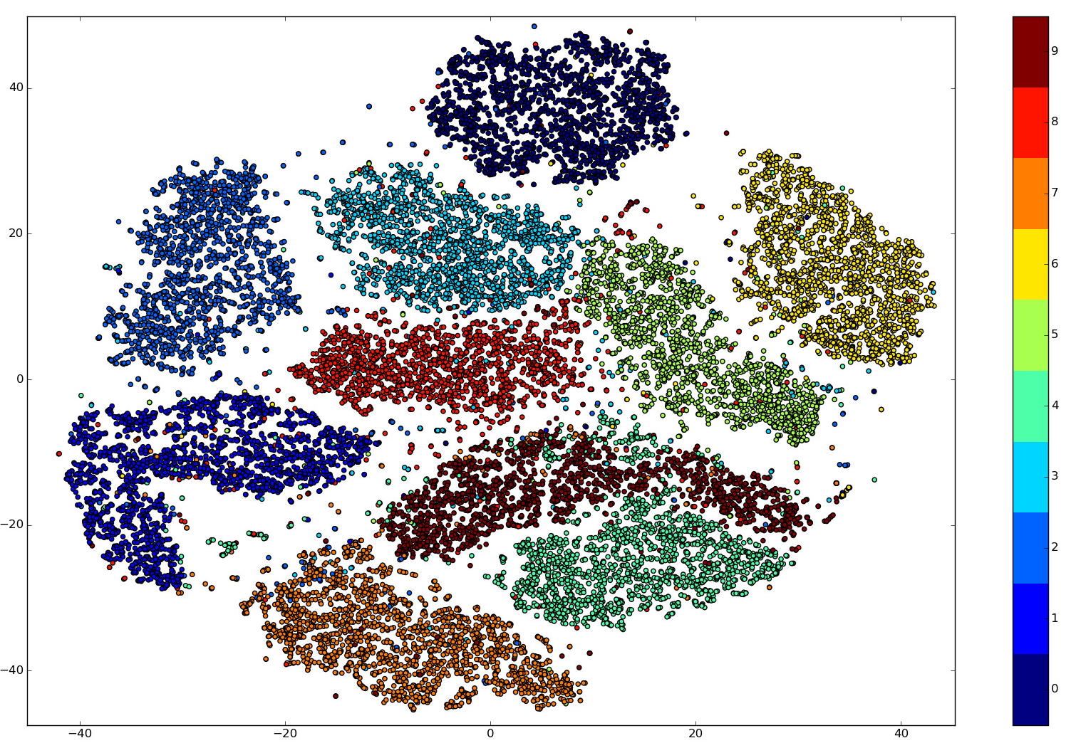
This approach to dimensionality reduction gives some truly excellent results. For example, on the well-known MNIST optical character recognition dataset, the t-SNE is already able to cluster the digits very well in two dimensions.
An example of this is shown in Figure 1 taken from a tutorial by Metz (2017) in Visualising with t-SNE. The algorithm shows the natural clustering of the images based on their digit. Considering that each image has dimensions of 28 multiplied by 28, the algorithm considers this to be a 282 dimensional vector; so the result is very good and corresponds well to how humans visualise these images.
Figure 1: Example of t-SNE applied to the MNIST dataset
Source: Metz L (2017), ‘Visualising with t-SNE'
Notes:
- The chart is taken from Visualising with t-SNE (Metz, 2017), accessed on 25 October 2017.
Download this image Figure 1: Example of t-SNE applied to the MNIST dataset
.png (1.9 MB)
Clustering using HDBSCAN
From our dataset, the expectation is that there will be lots of small clusters of business descriptions where similar business types have described themselves in a similar way. To effectively capture these clusters, we wish to identify the clusters based on the localised density of points in the vector space, rather than a cruder nearest neighbour method such as k-means.
HDBSCAN is a hierarchical, density-based clustering algorithm developed by Campello and others (2015), which builds on DBSCAN from Ester and others (1996). DBSCAN sorts three types of points: core points, on the interior of a cluster; noise on the exterior of a cluster; and border points on the boundary of a cluster. If we let D ∈ Rd then a point is distinguished by the parameters ϵ and MinPts. We define Nϵ (p,D):={q ∈ D∶|pq|≤ ϵ} to be a neighbourhood of a point p. A point p is a core point 8 if |Nϵ (p;D)| > MinPts, and a non-core point q is a border point if it is in the neighbourhood of a core point; else it is noise. Ester and others define the DBSCAN clusters based on the idea of density-reachability, which is detailed in their article, A density-based algorithm for discovering clusters in large spatial databases with noise (PDF, 616.6KB).
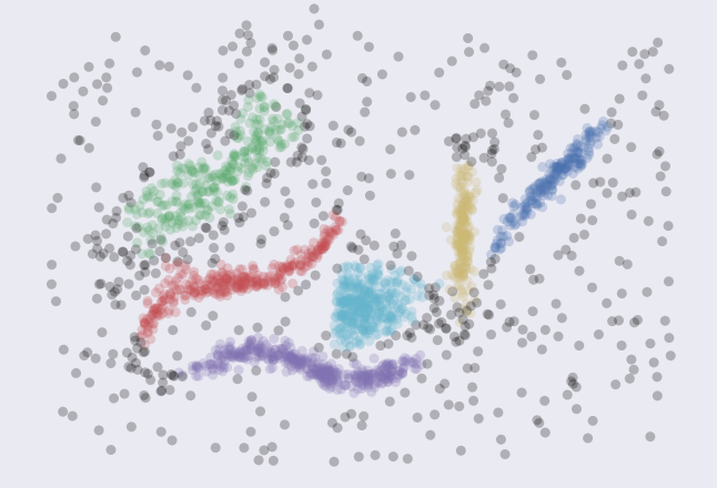
The advantage of using this algorithm is that it is very adept at accurately picking out clusters based on their density and connectedness rather than a nearest neighbour approach such as k-means clustering. This is demonstrated in Figure 2, with each cluster colour-code and noise represented as grey.
Figure 2: Example of HDBSCAN clustering
Source: Office for National Statistics
Download this image Figure 2: Example of HDBSCAN clustering
.png (149.1 kB)
Cluster topic extraction using singular value decomposition
The final stage of the pipeline is to try to identify a general topic that represents each of the clusters. If the clusters are very representative of the data within the cluster and not too noisy, then one possible way to extract a description of the matrix would be to find a low rank approximation of the matrix. If a rank 1 vector representation of the matrix can be found, the resulting vector can then be inferred back into the Doc2Vec model and we can imply a cluster topic based on the nearest document vector in the model to the inferred vector under the cosine distance.
To do this, a singular value decomposition (SVD) of the matrix can be found. The SVD is arguably the most well-known result from linear algebra and is a very useful matrix decomposition for a number of reasons; in this case, because it provides the best low rank approximation of a matrix under the Frobenius norm.
Let M be a m × n matrix, whose entries are real (although they can also be complex). Then there exists a singular value decomposition of M such that:
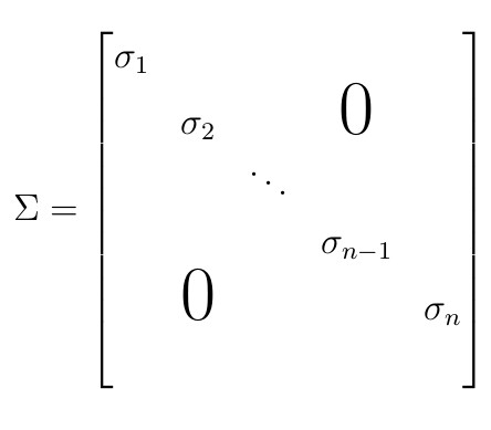
where U is an m × m orthogonal matrix, V is an n×n orthogonal matrix and Σ is a m × n diagonal matrix. The columns of U and V are known as the left and right singular vectors respectively and the structure of Σ is shown in Figure 3.
Figure 3: Matrix structure of sigma
Source: Office for National Statistics
Download this image Figure 3: Matrix structure of sigma
.png (10.0 kB)
The non-zero entries of M are ordered such that σ1 ≥ σ2 ≥ ⋯ ≥ σn. These are known as the singular values of M, where their roots are the eigenvalues of M. If we denote U = [u1 u2 … um] and V = [v1 v2 … vn], then we can see that the SVD decomposes M into the sum of rank 1 matrices weighted by its singular values such that:
In this case, we can construct a k-rank approximation of the matrix M by taking only the first k singular values of the matrix. In this case, we have the k-rank approximation as follows:
This is the best k-rank approximation to M under the Frobenius norm.
Back to table of contents5. Proof of concept results
First a Doc2Vec model was created using the full dataset of nearly 87,000 documents; that is, paragraphs describing businesses as described in section 2. This embedded each document into a 500-dimensional vector space. The research by Mikolov and others (2013a) suggests that when training the model, a dimensionality of between 300 and 1,000 dimensions works well. To give insight into how well the model has been clustering, some document vectors were inferred into the model and the nearest vectors (by cosine distance) in the model were outputted. If the model is providing meaningful results, we expect the nearest vectors to be similar to each other and the inferred vector, that is, there are clusters around the inferred vector.
To test this, we tested the string “elderly disabled care”; here Doc2Vec infers a vector and we can check the nearest documents to the vector. The results were as follows:
the principal activity of the company continued to be that of the provision of long-term care to the elderly and young disabled
the principal activity of the company during the year was the provision of residential care services for the elderly and disabled
the principal activity of the company during the year was the operation of a hotel for the disabled
the principal activity of the company during the year was residential care for the elderly and disabled
the company's principal activity during the year was that of sales and servicing of the equipment for the disabled
This shows the model is working well; the inferred vector is close to a group of documents that are represented very well by the phrase "elderly disabled care". This also suggests the model has clustered similar documents very well too. As well as being quality-assurance, this method of inferring vectors into the model may be useful in and of itself; for example, to find businesses that are engaged in a particular economic activity of interest. It should be noted that if a new string contains a vocabulary that is completely disjointed from the dictionary the model was trained on, the model will not know what to do as it has not seen that information. In this case, it initialises a random vector and so the result would be meaningless.
We can now visualise this using t-SNE as described in section 4.
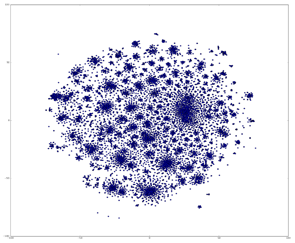
Figure 4: Dimensionality reduction using t-SNE
Source: Office for National Statistics
Download this image Figure 4: Dimensionality reduction using t-SNE
.png (450.5 kB)
Figure 4 illustrates the vector space in two dimensions after dimensionality reduction. We can now see there seems to be many small clusters of documents grouped together. We cluster this based on their densities using HDBSCAN, described in section 4.
Figure 5: Density-based clustering using HDBSCAN

Source: Office for National Statistics
Download this image Figure 5: Density-based clustering using HDBSCAN
.png (388.6 kB)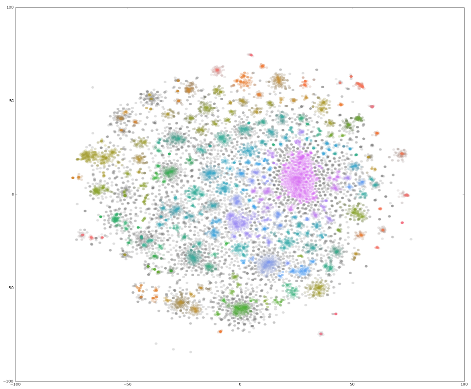
Figure 5 colour codes the different recognised clusters. In this case, although it is hard to visualise such a spectrum, HDBSCAN identified over 4,000 separate clusters containing at least two businesses. If we investigate business descriptions around these clusters, we get some interesting results. The following paragraphs present examples of three clusters and business descriptions within those clusters.
Cluster 1
Principal activities – the company is a wholly-owned subsidiary of a group whose principal activities are that of development and management of solar farms.
Principal activities – the company is a wholly-owned subsidiary of a group whose principal activities are that of development and management of solar farms.
Principal activities in the year under review is that of the development, construction and operation or sale of wind farms; provision of commercial asset management services to wind and solar farms and provision of operational management services to wind farms.
Cluster 2
The principal activity the principal activity of the company is to provide student residential accommodation.
The principal activity the principal activity of the company is to provide student residential accommodation.
The principal activity the principal activity of the company is to provide student residential accommodation.
Cluster 3
The company's principal activity is providing data storage services and solutions.
The company's principal activity is providing data storage services and solutions.
The principal activity of the company was that of an independent integrator of data storage and data management solutions.
As we can see, through exploration of the clusters, different business classification topics can clearly be identified. This will not always be the case; for instance, some of the larger clusters will contain noise where the model is picking up certain phrases that are not related to the business activity. These examples also pick out some types of business activity that may be of particular interest as they pertain to new kinds of economic activity.
With the recent explosion in big data, cluster 3 shows a cluster containing businesses selling data storage and management solutions. Cluster 2 shows an emerging area in the private lettings of student accommodation, another relatively new type of business activity. The model also picks out established industries very well, such as banking, property or, for example, in cluster 1 the production and maintenance of solar farms.
With large amounts of data and clusters, generally we will not want to manually give each cluster a topic. If we assume that the data are very similar within clusters, this justifies the use of singular value decomposition. Here we collect a separate matrix containing the document vectors for each separate cluster. We then take an SVD of each cluster's document matrix and return a rank 1 vector representation of the matrix. The vector can then be compared via the cosine distance to all other documents in the Doc2Vec original vector space, and the closest vector is returned. This document can be used to describe the cluster as a whole, or a topic can be manually inferred from the document description. The technique can be used to automate cluster topic identification, especially when – like in this case – there are thousands of clusters and manual labelling is prohibitive.
The results for the three example clusters shown earlier are as follows:
Cluster 1:
Cluster topic: principal activities – the company is a wholly owned subsidiary of a group whose principal activities are that of development and management of solar farms.
Cluster 2:
Cluster topic: the principal activity the principal activity of the company is to provide student residential accommodation.
Cluster 3:
Cluster topic: the company's principal activity is providing data storage services and solutions.
The topic descriptions are each very representative of the clusters shown as they each relate to a business within the cluster. From this process, it has been shown that using the proposed machine learning pipeline, an automated, unsupervised machine learning process can be used to cluster documents and also infer a cluster topic.
Back to table of contents6. Discussion and further work
From the results we can see that this methodology of creating a document vector space using Doc2Vec, followed by dimensionality reduction, clustering and singular value decomposition, produces meaningful results. In general, the final result will depend on a few different areas. First, we have trained the Doc2Vec model using a relatively small amount of data in big data terms. Although this seems to be sufficient to produce meaningful document embeddings, to produce results with more confidence a large training set would be needed. With an insufficient amount of data to train with and poor preprocessing of the documents, this may not produce a sufficient result. Parameters can also be tuned with both dimensionality reduction and clustering algorithms too; t-SNE can be tuned to focus on local or global information and similarly, HDBSCAN can be tuned to ignore small clusters. If a cluster is too noisy, then the singular value decomposition of the cluster's document matrix may not be sufficiently representative as it may pick out a noisy vector. This is a consequence of the model not being well trained rather than using the SVD approach.
In our application, although the model has produced meaningful embeddings, a lot of the clusters are dominated by popular business types, such as holding companies, financial services and property management and investment. To really capture some more granular business information, we conclude that more data are needed to train the model. Despite this, the model provided some interesting insights about the economic activity of UK businesses. The model can pick out some emerging trends and showing potential misclassification. It is also useful to explore business types by inferring a vector into the model; so for instance, if we are interested in renewable energy, we can create a vector of some key words and discover businesses close to that description.
We are currently in the process of obtaining a richer source of data, which we intend to use to publish research using automatically-generated classifications alongside Standard Industrial Classification 2007: SIC 2007 to measure aspects of the UK economy. Methodologically, the pipeline can be further extended to categorise businesses based on the document vector space embeddings. This vector space could be used as a feature space for machine learning classification.
Back to table of contents7. Pipeline Jupyter Notebook
A Jupyter Notebook showing an example of this pipeline using the data extracted from Companies House is available.
Back to table of contents8. References
Bean C (2016), ‘“Independent review of UK Economic Statistics’, Office for National Statistics
Companies house archive (accessed on 25 September 2017).
Mikolov T, Chen K, Corrado G and Dean J (2013a), ‘Efficient estimation of word representations in vector space’, CoRR
Mikolov T, Sutskever I, Chen K, Corrado G and Dean J (2013b), ‘Distributed representations of words and phrases and their compositionality’, CoRR
van der Maaten L and Hinton G (2013), ‘Visualising data using t-SNE’, Journal of Machine Learning Research, volume 9
Campello RJ, Moulavi D, Zimek A, and Sander S (2015), ‘Hierarchical density estimates for data clustering, visualization, and outlier detection’, ACM Transactions on Knowledge Discovery from Data (TKDD), volume 10, issue 1, page 5
Ester M, Kriegel HP, Sander J and Xu X (1996), ‘A density-based algorithm for discovering clusters in large spatial databases with noise’, Proc. 2nd International Conference
Metz L (2017), ‘Visualising with t-SNE’, accessed on 25 October 2017
Back to table of contents